The demand for generative models is rapidly increasing. Particularly, generating realistic, safe, and useful tabular data is crucial for industries, wherein this type of data is most common. Among the direct applications of tabular data generation we can cite data privacy, imputation, oversampling, explainability or simulation [1, 2]. Because of their ability to learn valuable data representations, another significant application of these models is pre-training and fine-tuning for various downstream tasks [3, 4, 5]. However, generating high-quality tabular data presents several technical challenges that are not encountered with text or images [6]. First, tabular columns are encoded through heterogeneous data types with distributions that are often non-smooth with mixed (continuous/discrete) behaviours and various modalities. There can also be complex dependencies between columns, and the categorical features are often highly imbalanced. Finally, the wide variety of problems represented in tabular form makes it challenging to establish a universal data encoding and architecture suitable for pre-training across all scenarios.

To handle these challenges, many models have been proposed in the literature, which are often evaluated on different datasets with inconsistent metrics, tuning and training budgets. Indeed, the performance of the allegedly best tabular generation models seem very unstable from one dataset to another. Moreover, these models seem quite sensitive to the feature-encodings and hyperparameter-choices made by the authors.

In this work we propose a unified evaluation benchmark for tabular data generation. Our main contributions are :

• We present the state-of-the-art and propose the following typology of the existing models : non-iterative and iterative neural, which groups auto-regressive and diffusion models; as well as non-neural models.

• We study the impact of dataset-specific feature encoding, hyperparameter and architecture tuning on tabular data generation models. For each model we answer the following questions: (i) is it worth optimizing the hyperparameters/preprocessing specifically for each dataset? (ii) can we propose a reduced search space that fits well for all datasets? (iii) is there a clear trade-off between training/sampling costs, and synthetic data quality?

• We benchmark 5 models that are representative of the recent literature on 16 datasets with a strict 3-fold cross-validation procedure. The datasets were chosen based on their size, purpose and diversity.

• We consider in our benchmark both extensive and limited-budget optimizations for each fold and dataset through hundreds of trials.

It is worth noting that this paper is not intended to be a survey. Rather, it benchmarks selected models for tabular data generation through meticulous fine-grained tuning. Previous surveys on tabular data generation are either focused on privacy [7, 8, 9, 10, 11, 12] or do not cover recent diffusion models [2, 13]. Most survey only report the author’s evaluations with default hyperparameters. A few benchmarks like [14, 11] perform hyperparameter search, with simple train/validation/test split, reduced search space, and small number of trials (usually from 20 to 50). Instead, we provide large-scale extensive benchmarks. We select representative models of the literature and we evaluate them on distinct datasets in cross validation, in which for each fold and dataset, we optimized the model’s hyperparameters, feature encoding, and architecture through hundreds of trials. Unlike previous work, our benchmarks compare not only the realism, the utility and the anonymity, but also the costs and the carbon footprint.

Finally, we analyze the results of these benchmarks and derive some interesting insights about the models. While diffusion-based models like TabSyn and TabDDPM [15] generally outperform other models when left unconstrained, they do not significantly surpass their simpler counterparts when tuning and training budgets are limited. This is because models that do not rely on Transformers have a smaller memory footprint, allowing for more thorough optimization within the same GPU budget.

The paper is structured as follows. First we present the models’ typology in Section 2. The benchmark’s challengers, metrics, datasets and other experimental settings are presented in section 3. The extensive and limited-budget benchmarks are detailed in Sections 4 and 5 respectively. Finally the conclusions is presented in Section 6 and the future work in Section 7.

Tabular data generation is a booming research field which gives birth every month to a host of new data synthesis algorithms. In this section we survey the existing families of tabular data generation methods with a specific focus on the models that we selected for our study. This includes models already covered in [2] and [13] as well as more recent diffusion-based models and LLM-based ones [16]. We chose models known for their strong performance, widespread usage, and availability of code that can be easily adapted for both architecture and hyperparameter tuning.

The following neural and non-neural approaches have been proposed for tabular data generation. Among the neural approaches, we make a distinction between the “push-forward” models which directly map noise into data, and the iterative models which require a decoding phase.

2.1. Non-iterative Neural Models

The most popular non-iterative or “push-forward” neural networks for tabular data generation are Variational Auto-Encoders (VAE) [17] and Generative Adversarial Networks (GAN) [18]. A few papers also consider selfnormalizing flows [19]. One of the simplest VAE architecture for tabular data is TVAE [20]. In its original implementation [21], it consists of a one-hot encoding for categorical variables coupled with a Gaussian Mixture Model normalization scheme (GMM) for continuous features. The encoder/decoder architecture is a simple stack of linear layers. Several variants have been proposed to improve from this baseline. In [22] the GMM normalization is replaced by a two-step training that first fits the marginals then fits the inter-dependencies. In [23, 24], several normalization schemes were tested as a replacement for the GMM normalization. Other variants of VAE use differentiable oblivious trees to ensure privacy [25]. In [26] the VAE is coupled with a Graph Neural Network (GNN).

The most popular method to generate tabular data is certainly adversarial training [27, 28, 29, 30, 31, 20, 32, 23, 33, 13, 34]. It would not be exaggerated to affirm that every exotic variant of GANs has been tested on tabular data generation, but the most successful architectures seem to be the ones based on Wasserstein GANs [35] such as CTGAN [20]. CTGAN is the base architecture that we selected for our benchmark. As mentioned in [23, 24], the feature encoding scheme is critical, especially for numerical features. For this reason we customized the CTGAN code as we did for TVAE, to allow for a choice of architecture and feature encoders.

2.2. Iterative Neural Models

It has been shown that iterative generative models (either auto-regressive or by diffusion) almost systematically outperform push forward models when it comes to raw text, sound, or image generation [36]. We confirm here that tabular data do not escape this rule. However, this performance comes with a cost: the decoding phase is often slow and highly energy consuming.

2.2.1. Auto-regressive Language Models

After the recent breakthrough of large language models (LLM) [37], the usage of token-based language models to generate tabular data seems inevitable. Their main advantage against prior ad-hoc models is that they come without specific feature encodings for numerical or categorical columns: these values are directly fed to the model as raw sequences of tokens. Even if there is no clear agreement yet on how tabular instances should be serialized for LLMs, this general encoding ability opens the possibility for a pretraining/finetuning paradigm on heterogeneous tabular datasets [3, 5].

In a recent preprint survey [16], the authors tried to map the exuberant flow of preprint papers on tabular data and LLMs. Several of these preprints present only prompt engineering tricks that generate small tables, nonetheless some of the proposed models seem promising at a larger scale. To name a few of them, GReaT [38] (for ”Generation of Realistic Tabular data”) proposes to fine-tunes GPT-2 [39] for tabular data generation. REaLTabFormer [40] extends GReaT to multiple tables with shared indexes, and TAPTAP [5] experiments a pretraining of GReaT on 450 open tabular datasets.

We made a few experiments with GReaT and its variants and confirmed the remarks of [15, 11], which state that they struggle to capture the joint probability distribution on datasets where the categorical values names do not carry semantic information. Given the prohibitive computational cost of LLMs, the large number of hyperparameters and serialization schemes to consider, as well as the problematic fact that some datasets are already covered (i.e. used in the training data) by the foundation models training sets, we decided to postpone their evaluation for a future work.

2.2.2. Diffusion models

Another recent impressing breakthrough in generative modeling, especially in image generation, was the apparition of diffusion models [41, 42, 43, 44, 45]. These models learn to iteratively transform random Gaussian noise to a sample from an unknown data distribution. This transformation is defined through a forward and a backward diffusion processes. The first one iteratively adds Gaussian noise to samples, while the second one iteratively “denoises” samples from the Gaussian distribution to obtain samples from the data distribution. The transposition of these models to tabular data gave rise to powerful synthesizers: TableDiffusion [46], Stasy [47], CoDi [48], and TabDDPM [14]. In TabSyn [15], a more recent proposal, the authors transposed the idea of [49, 50] to make use of a transformer-based VAE in order to embed the diffusion in a latent space. We selected both TabDDPM and TabSyn for our benchmark.

2.3. Non-neural Models

The most common statistical approaches are based on copulas and Probabilistic Graphical Models (PGMs). Copulas [51] are functions that join or “couple” multivariate distribution functions to their one-dimensional marginals. They have been widely adopted for tabular data generation because they allow modeling the marginals and the feature inter-dependencies separately [21, 52, 53, 54, 55]. Nevertheless, parametric copulas have been shown to perform poorly on high-dimension data synthesis problems [20, 24].

On the other hand PGMs can model variable dependencies in high-dimension spaces [56, 57, 13, 58, 59, 60]. This approach has been shown to be quite efficient in the data privacy community [61, 9, 10, 11]. However, it often requires a prior knowledge on the dependency graph because graph inference from data is inefficient in high dimension, especially if the sample size is small [62].

The fact that ensembles of trees remain state of the art for predictive tasks on tabular data [6] motivated some interesting attempts to mimic the neural generative approaches with decision trees. It gave rise to adversarial forests [34], Forest-Flow, and Forest-VP (a variance-preserving diffusion algorithm) [63]. We tested Forest-VP but we encountered a severe scalability issue: contrary to neural diffusion models, introduced in Section 2.2.2, where the noise level is combined with the input as an auxiliary variable, the Forest-VP algorithm trains a different ensemble of trees for each level of noise.

Another simple, but quite efficient way to generate new tabular data is to interpolate between existing instances. This geometric “nearest neighbors” approach called Synthetic Minority Over-sampling Technique (SMOTE) [64, 65, 66] is frequently used to resample instances before training predictive models on unbalanced datasets. It proceeds by picking a random instance with a fixed target value and finding its k nearest neighbors. New data points are then generated by interpolation between these neighbors. Although very simple, this model is a solid baseline for tabular data generation as shown in [14].

We first present the selected challengers and the various evaluation metrics. Then, we present the optimization framework that we developed and we discuss the choices made to wrap the different challengers into this framework. Finally, We present the datasets.

3.1. Selected Challengers

We selected five models for our benchmarks, two iterative neural: TVAE, CTGAN; two diffusion models: TabDDPM, and TabSyn; and one non-neural: SMOTE (with a variant unconditional SMOTE, namely ucSMOTE). We followed [24] and used a customized version of TVAE which allows for an optimized choice of the architecture and of the feature encoder.

For each of these algorithms we had to carefully examinate the code to optimize large scale hyperparameters, features encoding and architecture. We also reported the trivial baseline which consists in resampling directly the train set, namely “

3.2. Evaluation Metrics

Our purpose is to assess the quality of tabular data generation though multiple facets. These facets can be summarized with four questions: (i) is synthetic data realistic? does it respect the original distribution’s traits? (ii) is it useful? i.e. can it be used to train machine learning models? (iii) do synthesis preserve training data anonymity? does it overfit? (iv) what are the model’s costs and COimpacts? Each of these questions is related to specific metrics.

The first and most important question is the realism of the generated data. We rely on (C2ST) [67] as a primary metric to address it. This metric is also the one that we used for hyperparameter optimization. It evaluates the performance of a classifier at discerning real data from synthetic data. To compute C2ST we use the same protocol as in [24] where the computed value is the mean ROC-AUC of XGBoost [68] over three folds. A C2ST around 1/2 means that XGBoost is unable to discern the test set from the generated set. A high C2ST means on the contrary that XGBoost is able to detect easily the fake data. The C2ST calculation procedure is summarized in Figure 1.

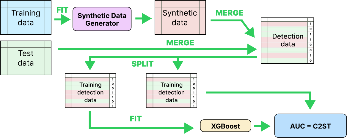
Figure 1: C2ST Metric calculation.

We also consider two other statistical metrics for data realism: column-wise similarity and pair-wise correlation. To compute these metrics we used the SDMetrics library [21]. The column-wise similarity measures how accurately the synthetic data captures the shape of each column distribution individually. It is reported as ”Shape” in the result tables. Pair-wise correlation on the other hand captures how each column varies with each other. Pair-wise correlation is reported as ”Pair” in the result tables. A naive generator that would assume independence of the columns might have a high ”Shape” score but it would have a low ”Pair” score.

The second important question is the utility of generated data. It is commonly measured by ML-Efficacy which evaluates the performance of a predictive model trained on synthetic data. To compute ML-Efficacy we use the same protocol as in [14] where CatBoost [69] is used as a predictor. We report the F1 score for classification tasks and the normalized R2 score for regression tasks. The procedure is summarized in Figure 2. It is important to evaluate the degradation of these scores against the ones obtained when training directly on real data (via Train Copy): a large degradation means a low utility.

The third question is anonymity. We want to make sure that our generative model will not leak sensitive information by recopying or over-fitting the training instances. To do so we measure respectively the minimum distances of each generated instance to the train and test sets. The Distance to Closest

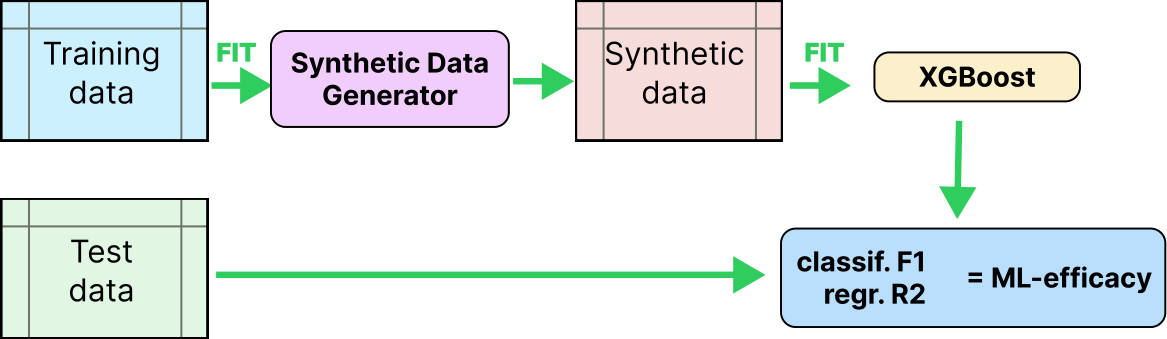
Figure 2: ML-Efficacy Metric calculation.

Record Rate (DCR-Rate) counts the proportion of generated instances that are closer to train set than test set [70]. The procedure is summarized in Figure 3.

A synthetic dataset is considered safe if it has a DCR-Rate that is close to 1/2. On the other hand, a plain copy of the train set, as Train Copy baseline does, would have a DCR-Rate of 1. This metric does not guarantee against all privacy breaches, but it provides a reasonable safeguard and ranking criterion for the models. It is also informative about overfitting, as an overfitted model would have samples that are systematically closer to the train set than a model with more generalization capabilities.

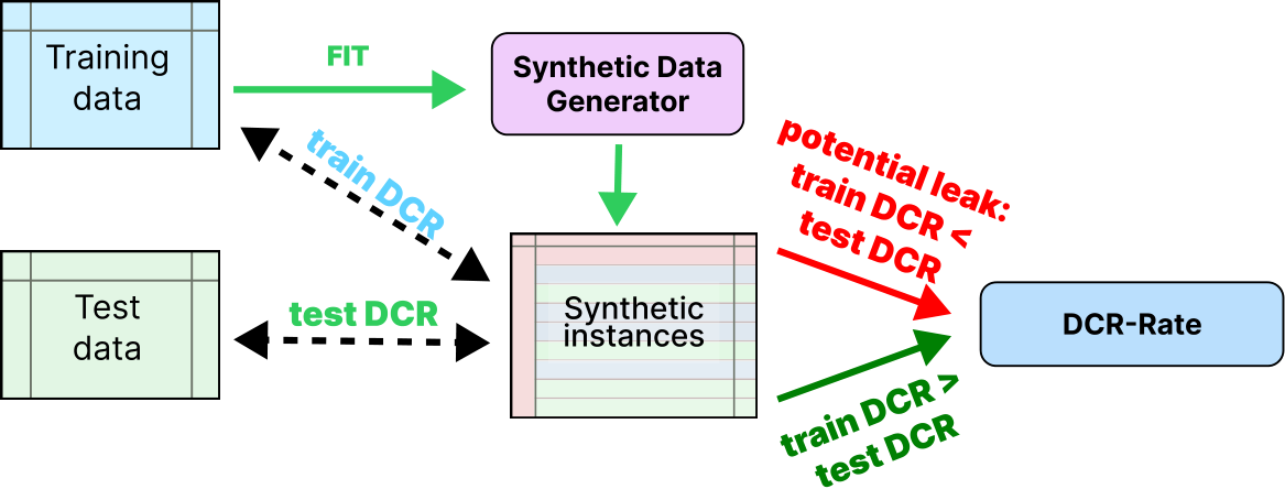
Figure 3: DCR-Rate Metric calculation.

It requires an accurate estimate of three cost values: time, energy consumption, and . Ideally, these values should be estimated for the three phases of (i) training (gradient descent) (ii) sampling, and (iii) hyperparameters search. For each dataset, each fold and each optimized model architecture, we ran the training and sampling phases on the exact same hardware and software architecture, a single Tesla V100 32 GB, and we measured accurately the cost values with the . However, due to the massive nature of the experiments, we could not perform the whole hyperparameter search and training phases on such a uniform hardware and software architecture. We hence estimated the global search costs from the tuning logs by rescaling the training cost measures according to the effective number of steps performed and the number of GPU used (c.f. equation (1)).

total-gpu-cost

This is slightly overestimated since: (i) CodeCarbon assumes a 100% GPUs load while ours was roughly around 95%; and (ii) we measured the step costs on already optimized models which are usually slower because they often count more layers and parameters. Note that the number of trials that can be parallelized on a single GPU depends on the memory footprint of the model

3.3. Large Scale Optimization Framework and Implementation Details

Providing a fair and reliable comparison of the different tabular generative models is a tough technical challenge. For this reason most existing benchmarks like [38, 15] only report the performance of models with their default hyperparameters. A few benchmarks like [14, 11] perform hyperparameters search for all models, but with a simple train/validation/test split, a reduced search space, and a small number of trials (usually from 20 to 50).

We wanted our experiment to be more extensive and more robust, so we decided to deploy it at a large scale on a super-computerequipped with several nodes with 4 GPUs V100 32GB each

For this purpose, we used the Ray tune distributed library [71] coupled with Hyperopt [72] which is based on Tree Parzen Estimators (TPE) [73] and Asynchronous Successive Halving Algorithm (ASHA) as a scheduler [74] to optimize hyperparameters and architecture efficiently. Depending on the

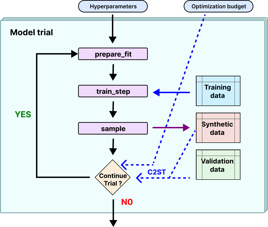
Figure 4: Hyperparameters trial optimization loop.

model’s memory footprints, each GPU could host from four to twelve concurrent tuning trials. For each dataset and each model we performed a strict 3-fold cross validation, which means that for each tuple (dataset, fold, model) we performed an extensive hyperparameters search with 300 trials (except for TabSyn where we reduced this number to 100 for technical reasons explained in Section 3.3.2). We hence obtained a different optimized architecture for each (dataset, fold, model) tuple.

In [14] the parameters were optimized for ML-efficacy, in [11] the parameters were optimized for an equal combination of realism, utility and privacy. We chose to optimize for realism as in [24] through XGBoost-based C2ST metric (c.f. Section 3.2). To obtain reliable evaluations with variance estimates, for each dataset we evaluated the models by averaging all the metrics on the three folds test sets with five synthetic samples for each fold.

As described in Figure 4, in order to work with our framework each algorithm has to be wrapped into a generic Synthesizer class that provides three methods: prepare fit which prepares the dataset and the model according to the hyperparameters, train step which performs a training step roughly equivalent to one or a few epochs, and sample which generates synthetic data. After each train step, the model trial was evaluated and it was canceled out by early stopping or by the Ray-Tune scheduler if it performed too poorly or if the time budget was depleted.

3.3.1. The importance of feature encoding

Table 1 presents the encoding schemes that we used for the different benchmark challengers. As pointed out in [6, 23, 24], categorical variables are not the main weakness of neural networks but numerical feature encoding is critical. Most recent neural models use a Quantile-based numerical feature encoding and seem to work well with it. However, the original versions of TVAE and CTGAN rely on a specific Cluster-Based normalization [20]. We hence explored several encoding policies for these two models through hyperparameters optimization (see Tables A.6 and A.7 in the appendix section).

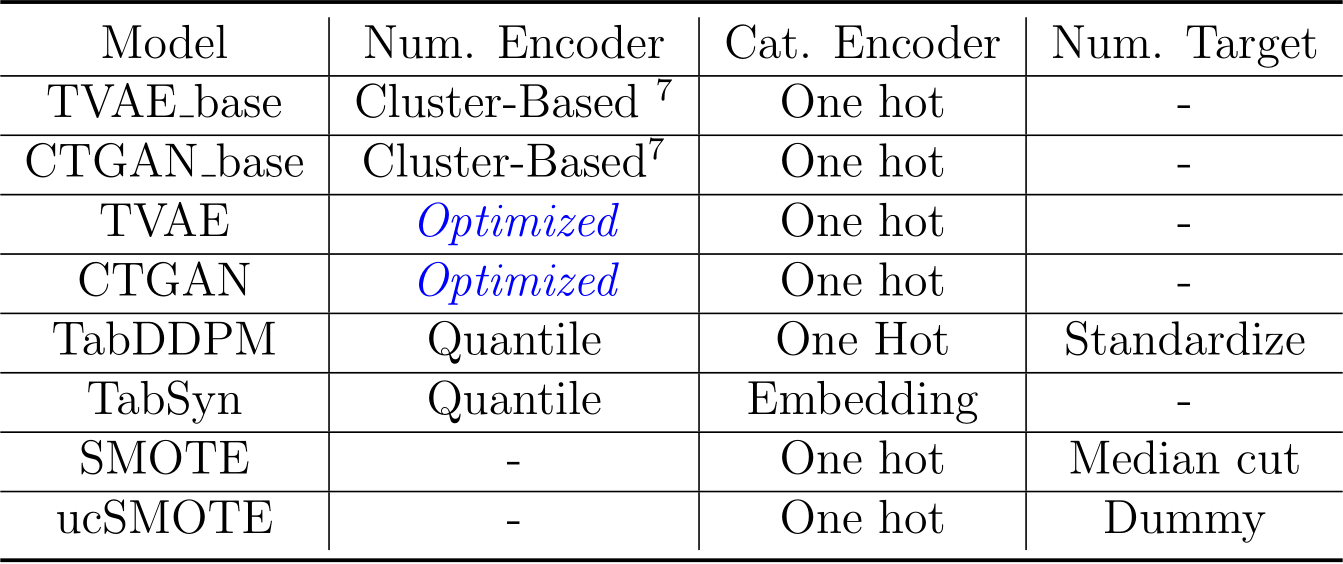
Table 1: Encoding schemes applied to TVAE and CTGAN.

We kept the native Cluster-Basedencoder as described in [20], along with the ones proposed in [24], namely: prototype encoding (PTP) [24],

piece-wise linear encoder (PLE) [75], continuously distributed residuals (CDF) [76, 24], hybrid (PLE CDF) [24]. We also added some standard scikit-learn transformers: MinMaxScaler and QuantileTransformer.

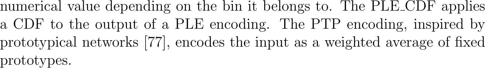
Contrary to QuantileTransformer which maps values deterministically, the CDF encoding uses randomization to produce continuously distributed residuals even when the original distribution is discrete or partially discrete [76]. The PLE encoder [75] performs a feature binning and normalizes each

3.3.2. Model-specific implementation details

Wrapping heterogeneous models within a Synthesizer class required some implementation choices from our part, and despite all our efforts to keep a fair comparison, these choices had some impact on the compute time and performance of the models.

The first issue is the discrepancy of the training step’s costs. The usual training step unit for most models is the epoch which corresponds to a single pass on all instances of the training set. However, depending on the hyperparameters some models like CTGAN perform both one pass through the generator and several passes through the discriminator at each training step. Other models such as TabDDPM are randomized and require several quick passes (almost one for each level of noise) for each instance. We hence had to caliber our wrapper’s train step functions to perform a compute effort that is roughly equivalent to an epoch.

Another issue is the fact that TabSyn [15] combines two models and was not designed for hyperparameters tuning. According to the authors the model does not need hyperparameters tuning. We decided to train a new transformer-based VAE for each trial because it hosts most of the parameters, compute-time and hyperparameters of TabSyn. Training a diffusion model on an unstable latent space would not be meaningful. We thus considered three technical options: (i) optimize first the VAE on a proxy metric (for instance the ability of its decoder to generate realistic data from a standard Gaussian), then optimize the denoiser in the latent space; (ii) wrap the VAE training steps into the train step function and retrain a new denoiser from scratch at each step; (iii) wrap the VAE training phase into the prepare fit function and loose the ability to prune its training steps. The first option is the cheapest and it is probably recommended for most practical applications, but it may be sub-optimal due to the proxy metric. The second option is extremely costly. We hence opted for the third option although it had a non-negligible cost. Indeed, we followed the recommendation of [15] to train the VAE through 4000 epochs which turns out to be huge knowing that most other models only utilized 400 epochs in our benchmark.

We also reduced the number of parallel trials per GPU because of the large memory footprint of the VAE’s transformers. As a consequence, for TabSyn we had both to reduce the number of trials to 100, and to work on a sample of the largest dataset (Covertype) to get the results in a reasonable amount of time. It is worth noting that despite these handicaps, the optimized TabSyn remained better than its non-optimized version. To avoid this experimental bias for the second experiment in Section 5.2, we constrained TabSyn’s VAE to use only 10 minutes for training. On Adult dataset, for instance, it resulted in roughly 560 epochs.

Finally, the last issue was the different ways the models deal with the target columns. A model conditioned on the target column may improve its ML-efficacy. TabDDPM and SMOTE implementations are natively conditioned on classification targets, while TVAE, CTGAN and TabSyn are not.

We did not modify TabDDPM, but we considered two variants in our experiment for SMOTE: the first, that we call SMOTE, follows the design of [14], it uses the train target distribution for classification datasets and a rough median split for regression targets (see Table 1). The second, that we call ucSMOTE (for unconditional SMOTE), adds a dummy target filled with zeros to the data before calling the SMOTE oversampling library. By doing so, all columns, including the original target, are considered equally.

3.4. Datasets

To evaluate the models, we picked datasets with various characteristics to assess their performances under different scenarios. Datasets were chosen to cover various sizes, dimensions, different types of tasks (regression, binary, and multi-class classification) and various types of features (numerical, categorical, or mixed). We also added Moons a well known scikitlearn synthetic dataset. The complete list of datasets and their characteristics is presented in Table 2. The Covertype dataset size was reduced for TabSyn tuning as follows: 27500 in the training set, 18333 in the validation set, and 9167 in the test set.

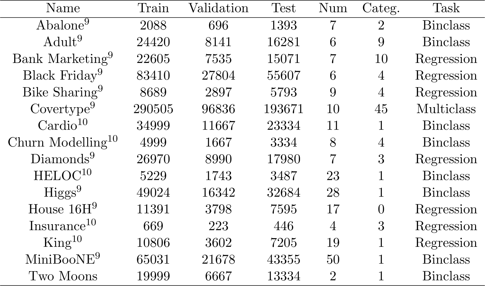
Table 2: List of datasets. Direct links to exact versions of datasets used can be found in Appendix B.

As mentioned in Section 3.2, the evaluation and comparison of tabular generative models is based mainly on four criteria: realism, usefulness, anonymity, and cost. After a global multi-criteria overview of the results, we study and compare the model’s behaviour according to each criterion individually.

4.1. Multi-criteria Overview

Figure 5 shows the average ranking over all datasets and folds of seven model variants over eight metrics (c.f. Section 3.2). To complete these rankings, Table 3 and Table 4 summarize respectively the quality metric and cost distributions among all datasets and folds. Recall that the best scores for the C2ST are around 0.50 (as it means poor AUC for the classifier at telling synthetic data apart from holdout data).

Overall, no model provides the best performance over all considered criteria. We observe, as expected, a strong correlation between energy and GPU time as well as a strong correlation among “quality metrics” (i.e. C2ST,

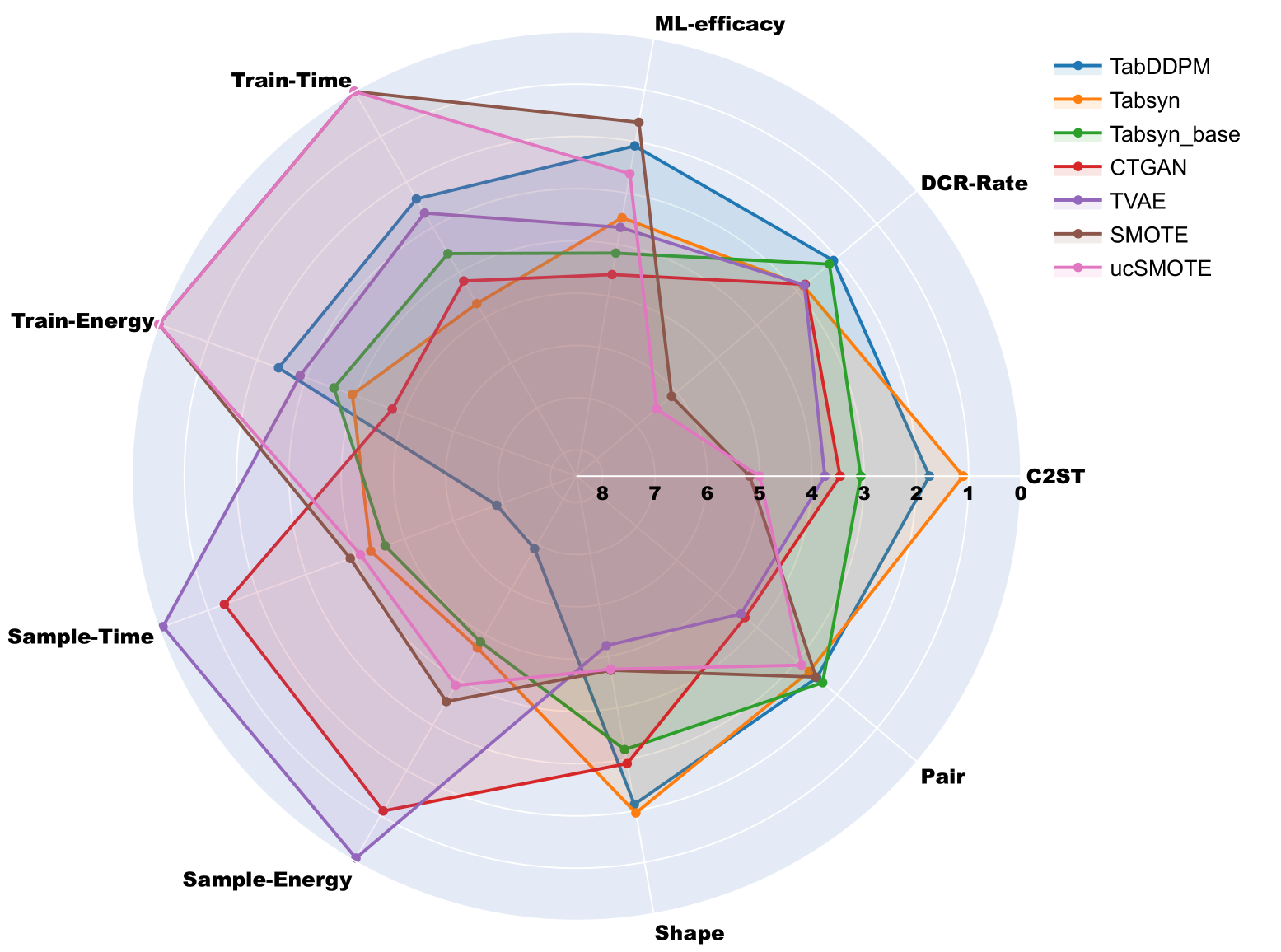
Figure 5: Radar chart of the extensive experiment showing optimized model’s average ranking on all datasets across various metrics. The training costs of optimized models include both tuning and gradient descent.

Shape, and Pair). On the one hand, the diffusion models achieve the best performance in terms of quality metrics, especially the tuned version of TabSyn. As shown in Table 3, this model has a median C2ST value of 0.64. However, TabSyn is also one of the most expensive models in term of training costs (Train-Energy as well as Train and Sample Times), as it requires to train both a transformer-based VAE and a denoiser model for each dataset.

On the other hand, the SMOTE baselines obtain the poorest quality and privacy ranking with a high DCR-Rate. The median DCR-Rate score for SMOTE and ucSMOTE is at 0.97 which means that most of the samples from these models are very similar to the training set. However, they achieve strong utility in terms of ML-Efficacy with quartiles very close to Train Copy and the same median value of 0.73. As expected for neighborhood-based algorithms, their training cost is negligible, but their deployment requires a neighborhood search which can be costly on large datasets. Finally the tuned neural push-forward models (CTGAN and TVAE) achieve mitigated results in term of both quality and utility but their deployment is clearly the cheapest. We also note that all neural models achieve reasonable results in term of privacy preservation. Although TabDDPM is clearly the slowest algorithm for deployment, it is fast at training and it obtains homogeneous results over all other metrics. We note that the tuned version of TabDDPM is performing better than the base version of TabSyn.

For this extensive experiment we only limited mildly the time budget and the number of epochs. However, some models like TabSyn and CTGAN consumed much more GPU time than others, especially TabDDPM which was very quick at performing an equivalent number of epochs (c.f. Section 3.3.2). It is also important to compare these algorithms with a fair allocation of GPU resource as we do in Section 5.

4.2. Detailed Analysis

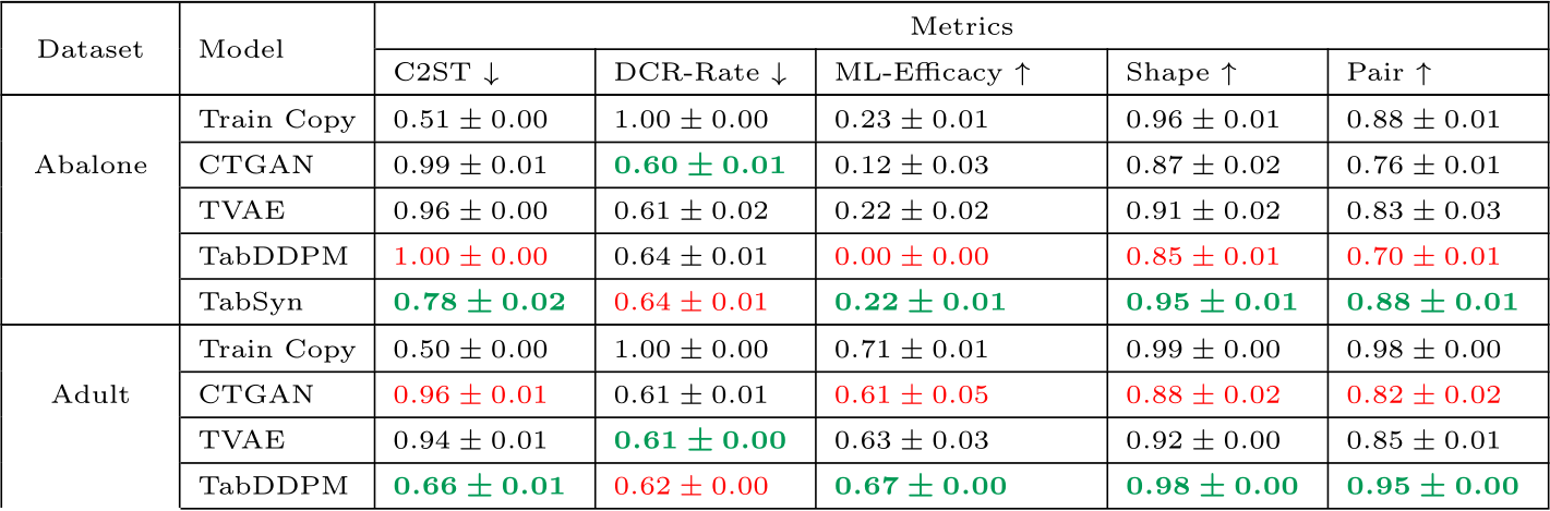
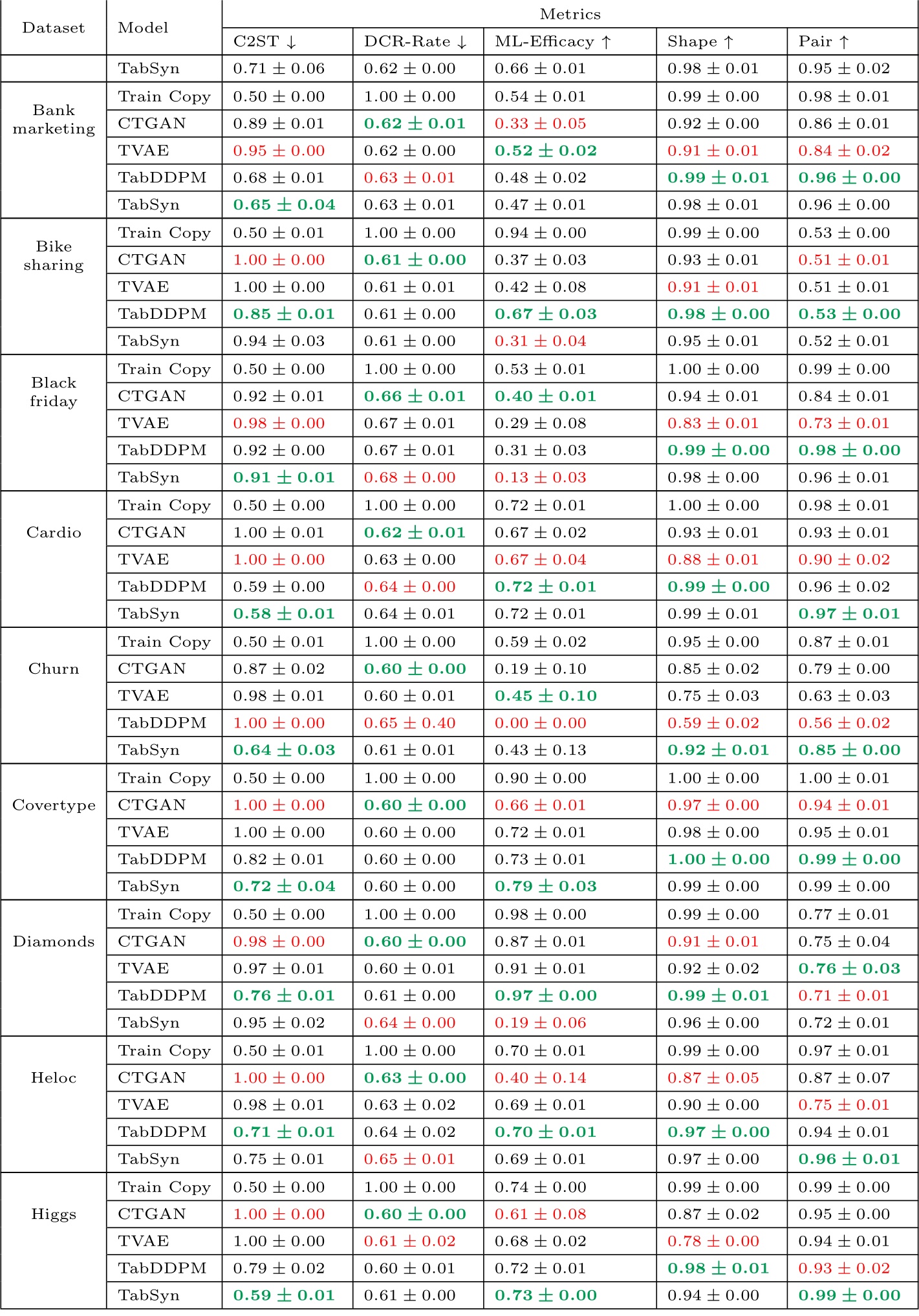
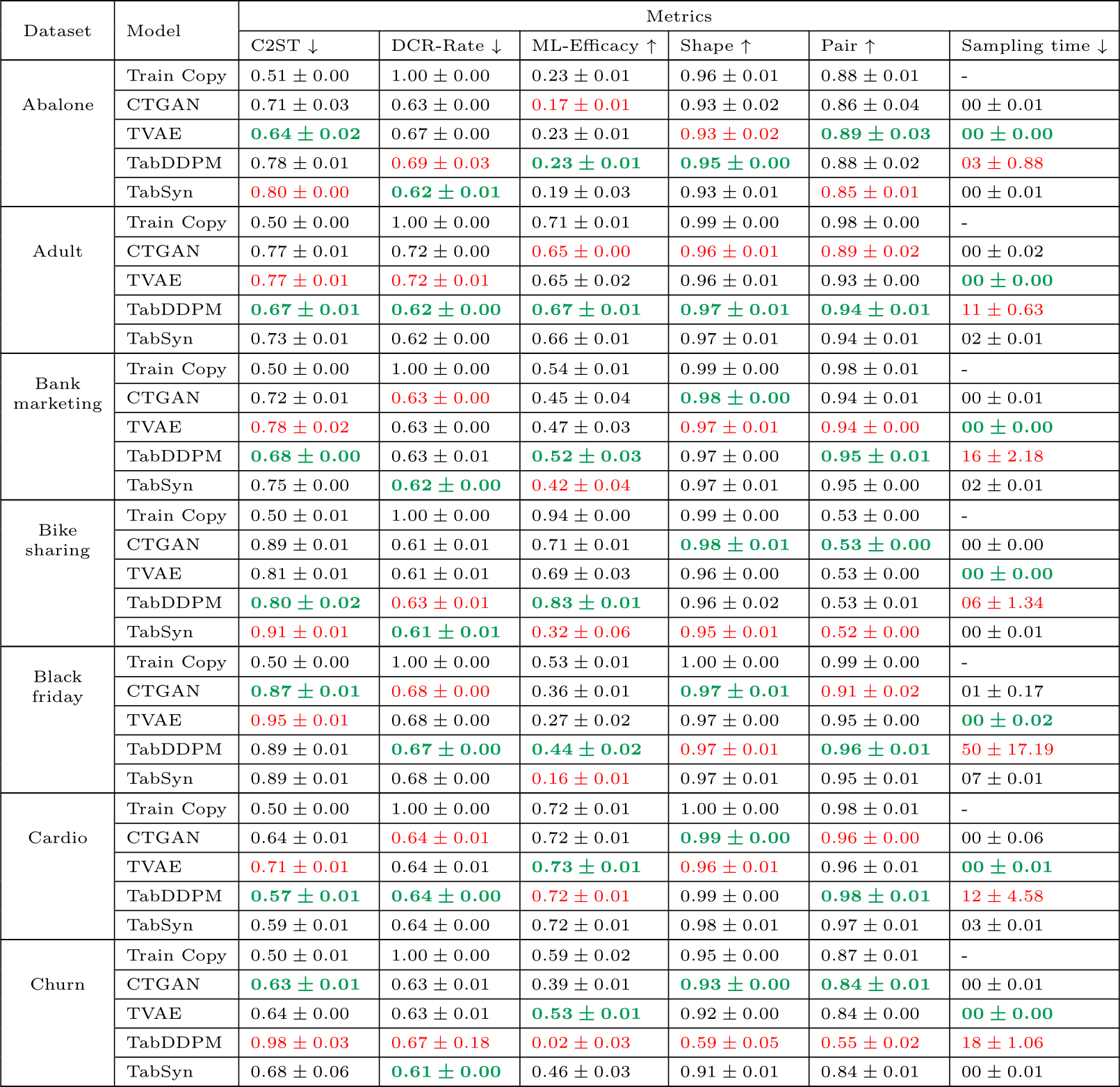
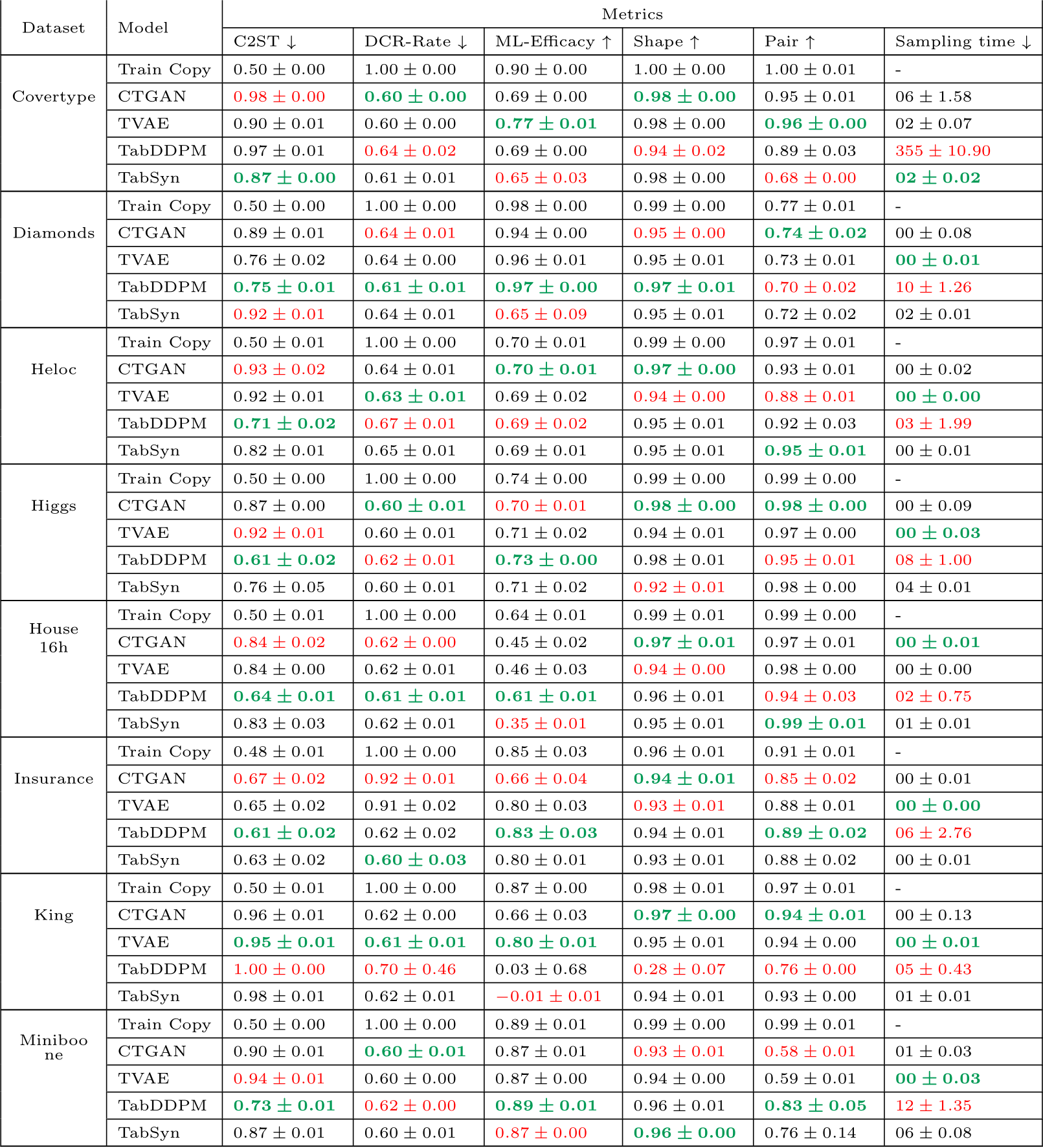
In this section we study and compare the model’s behaviour according to each criterion taken individually. For each dataset we computed the performance metrics over 3 folds and 5 synthetic samples per fold to provide a stable central tendency and dispersion estimate. The full dataset-level results are provided in Appendix Table C.12. We summarize these results among all datasets and folds in Table 3 and Table 4. For quality metrics we compare the models through critical difference diagrams.

4.2.1. Are synthetic data realistic ?

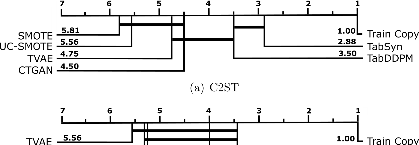
We show in Figure 6 the critical difference diagrams [78] of all tuned models respectively for C2ST, pair-wise correlation and column-wise similarity. These diagrams were obtained by aggregating the ranks of the seven models over all datasets and folds. A thick horizontal line groups the set of models for which the pairwise “no significant difference” test hypothesis could not be rejected.

If we except the trivial Train Copy policy which is by construction the most realistic generator, we note that TabSyn is significantly better in terms of C2ST than all other models except TabDDPM. On the other side, the SMOTE baselines are significantly worse than TabDDPM and TabSyn. The absolute C2ST values in Table 3 corroborate these ranking results with three sets of models: (i) diffusion-based models TabSyn and TabDDPM with a C2ST lower than 0.80 on most datasets and median around 0.65;

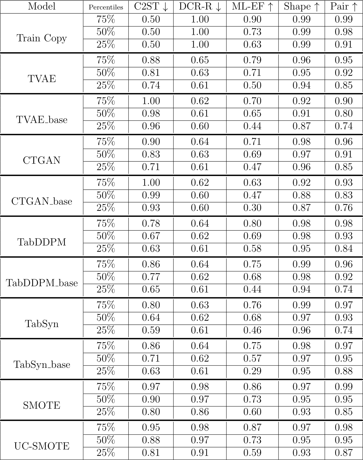
Table 3: Summary results from the extensive benchmark and the base models (i.e. with default hyperparameters), DCR-R stands for DCR-rate and ML-EF for ML-Efficacy.

3.44 3.44 TabSyn TabDDPMSMOTE UC-SMOTE

3.62 3.75 TVAE 5.56 5.50 4.19 UC-SMOTE

Figure 6: Models ranking with critical difference diagrams for C2ST, pair-wise correlations, and column-wise metrics over all datasets.

(ii) push-forward models CTGAN and TVAE with a median C2ST around 0.82; (iii) SMOTE algorithms with a C2ST higher than 0.80 on most datasets.

The rankings obtained according to the column-wise similarity are broadly the same as the one obtained for C2ST. In addition to the rank shown in Figure 6(b), we can see that all the models obtain good scores (usually around 0.96) as compared to the Train Copy baseline (0.99). This result suggests that all the models succeed at capturing univariate distributions. For pair-wise correlation, we note surprisingly high values for SMOTE and ucSMOTE baselines while the neural network models obtain broadly the same ranking as for C2ST but the gaps between models are less marked.

A side takeaway from this result is that XGBoost-based C2ST provides a stronger discriminative power than column-wise similarity and pair-wise correlation metrics.

4.2.2. Can the synthetic data be used to train a machine learning model ?

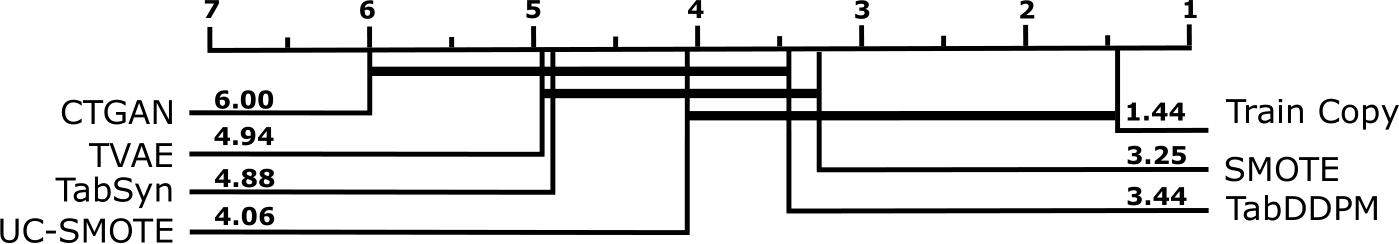
Figure 7: Models ranking with critical difference diagram for Catboost MLEfficacy over all datasets.

According to the machine learning efficacy metric (ML-Efficacy), the most useful generators are the ones that are conditioned on their targets (namely SMOTE and TabDDPM) with median values respectively at 0.73 and 0.69 (against 0.73 for Train Copy).

TabDDPM outperforms both base and tuned versions of TabSyn for this metric. It is also safer than SMOTE and it performs its training iterations faster than the other evaluated models. If ML-Efficacy is of importance, it is advisable to use this model. As expected, all models are far from the performance obtained on real data (Train Copy).

4.2.3. Does synthetic data preserve anonymity?

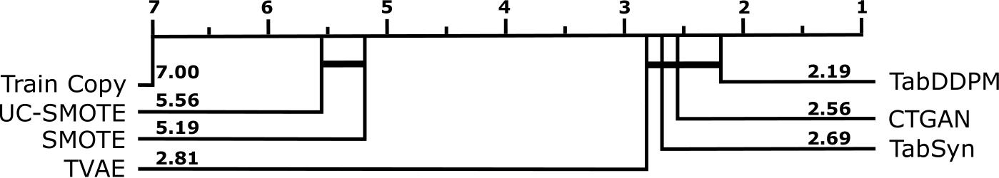
Figure 8: Models ranking with a critical difference diagram for the DCR-Rate metric over all datasets.

A data synthesizer that would only copy its training set would be of little value. If it generates new instances that are too close to its training set, it would obtain a good C2ST score, but it would be prone to over-fitting and it would leak private information from the training set. We assess the ability of a model to generate new data through the DCR-Rate metric (c.f. Section 3.2).

On Figure 8 we observe two significantly distinct groups of models. On the left-hand side a ”leaky” group that contains both SMOTE and ucSMOTE, and on the right-hand side, a ”safe” group that contains all neural algorithms. The poor performance of SMOTE is mainly due to the way it generates new data points by interpolating between existing ones. Therefore, these models cannot be considered safe concerning data protection. By taking a look at Table 3, the DCR-Rate of the two SMOTE variants is almost always above 0.86. On the other hand, if we exclude the tiny ”Insurance” dataset where CTGAN and TVAE overfitted, the DCR-Rate values of the ”safe” group are quite uniform around 0.62 and almost always below 0.65: these models can be considered safe.

4.2.4. What are the models’ costs?

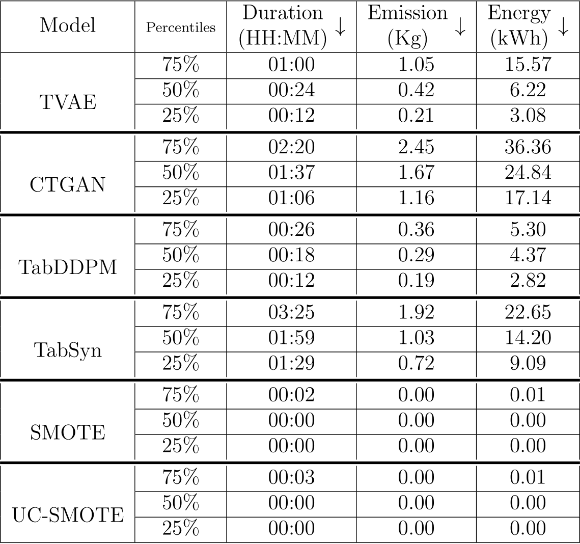
Table 4: Summary of the costs of the extensive benchmark. Costs dispersion of the 25th, 50th, and 75th percentiles are provided over all datasets and folds.

Model training, optimization, and data sampling have a cost and an environmental impact that varies greatly from one model to another. We hence measured and estimated time, energy consumption, and COfor each model during three phases: (i) training (measured), (ii) hyperparameters search (estimated), and (iii) sampling (measured). These results are reported fully in Appendix D. We summarize the tuning and training process cost distributions over all datasets and fold in Table 4. As mentioned in Section 3.2, these values are estimated from the tuning logs by taking into account the effective number of training steps, the number of trials, and the average GPU resource usage per training step as reported in Table D.13.

With a median tuning time around 18 minutes as shown in Table 4, TabDDPM is the fastest neural model. As a result, it also consumes less energy and it has less emissions at the training stage. As shown in Figure 5, considering its other performance metrics, it is a suitable choice to achieve good results at a relatively low training cost.

As expected, Figure 5 shows that the push models CTGAN and TVAE are the fastest at sampling stage. We notice that although CTGAN achieves slightly better quality results than TVAE, it is also one of the costliest models at the training stage as shown in Table 4. In order to achieve reasonable performance while reducing training costs, TVAE is hence an option to consider prior to CTGAN.

The training and tuning of TabSyn is one of the most demanding (with a median time of of 2 hours for tuning). In the end, however, it delivers the best performance in terms of quality metrics. This model also has the advantage of providing a set of default hyperparameters that can have a reasonable performance although, if we follow the author’s recommendation of 4000 VAE epochs, its training remains costly by comparison to other models. Indeed, Figure 5 show that, even if we consider the whole tuning+training pipeline TabDDPM and TVAE remain cheaper to train than TabSyn base.

In terms of sampling cost, TabDDPM is the worst-performing model. It takes longer than the other models (c.f. Figure 5) and hence consumes more energy with more COemissions at this step. TabSyn reduces the number of denoising steps by using VAE embedding and linear noises to reduce its sampling time [15]. It hence achieves better performance at inference than TabDDPM.

The two baselines SMOTE and ucSMOTE being based on neighbourhood interpolation their training and tuning cost is negligible. However, as shown in Appendix Table C.12, their sampling process requiring a nearest neighbor search, it is slower on large datasets than push-forward models like TVAE or CTGAN.

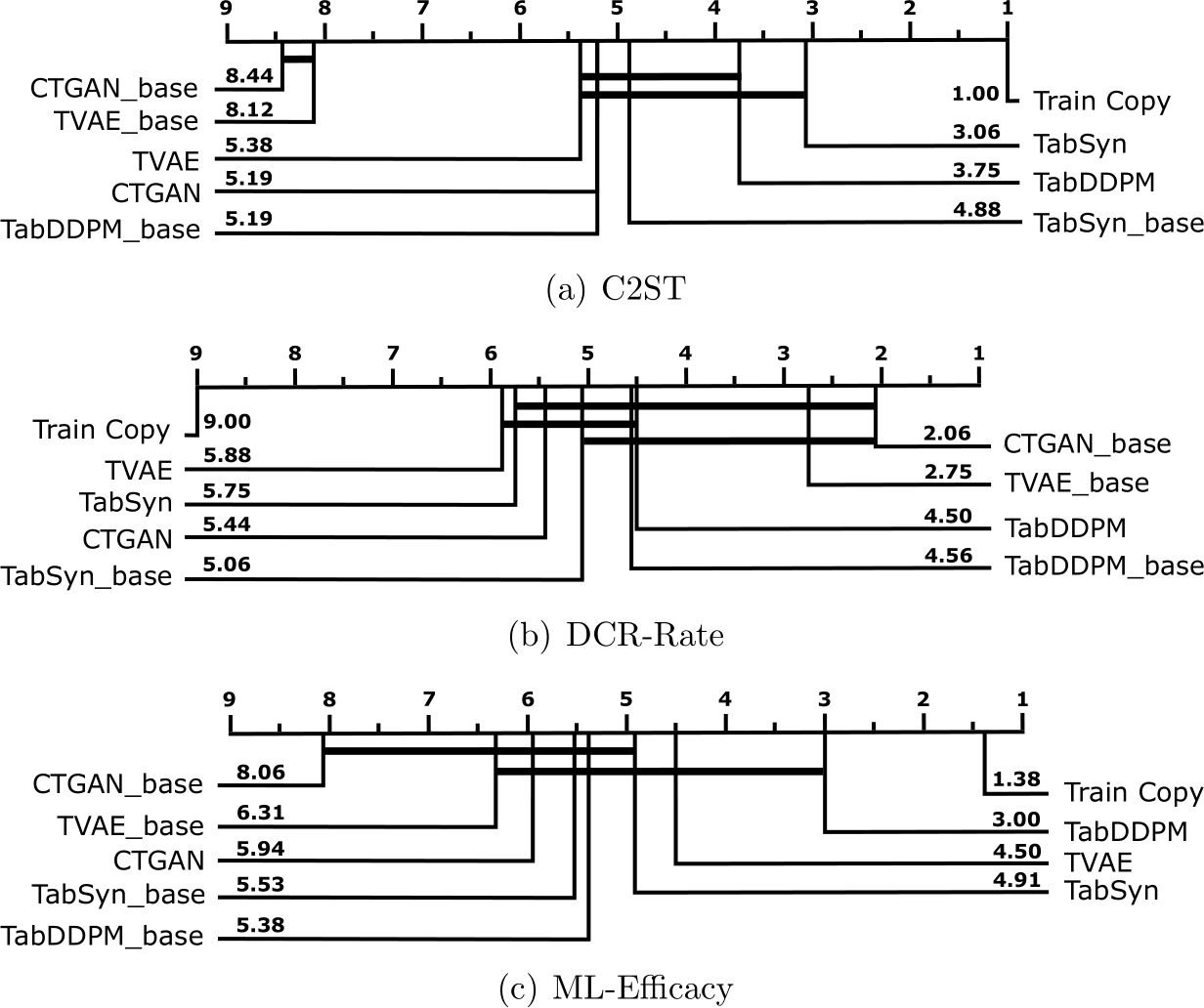
Figure 9: Models’ ranking with critical difference diagrams on C2ST, DCRRate, and ML-Efficacy metrics over all datasets: base models (i.e. with default hyperparameters) versus extensively tuned models.

4.3. Is it worth optimizing the hyperparameters for all models ?

As mentioned in the previous section, even with the help of sophisticated search algorithms, hyperparameter tuning is costly and the performance-versus-tuning-budget curve is following a diminishing returns law. We were hence interested in comparing heavily tuned models against non-tuned models.

To assess this, we trained the neural models using the hyperparameters provided by the authors in the original papers. These results are detailed in Appendix E.

In Figure 9(a) we can see a, sometimes huge, C2ST performance improvement of all models when tuned. This improvement is statistically significant between optimized TVAE and CTGAN and their base versions. Looking at the absolute C2ST values in Table 3, it confirms that these models should not be used with their default hyperparameters.

For TabDDPM and TabSyn, we also notice a 10 points improvement on the median C2ST but this gap is not large enough to provide statistical guarantees.

Although it was not the main target for tuning, we also observe an MLEfficacy gain for all models. This gain is marked at the 25percentile (i.e. for the hardest datasets).

We can therefore conclude that for all neural tabular generative models that we considered (including TabSyn), it is worth optimizing the hyperparameters specifically for each dataset if we want to improve performance. But the trade-off between the optimization cost and the performance gain is highly correlated to the size and design of the hyperparameter’s space (c.f. Appendix A). In the next section we propose a reduced search space and study the impact of a ”light” hyperparameters optimization with a limited budget.

As underlined in Section 4.3, optimizing the hyperparameters for each dataset can significantly improve the quality of the generators. But a large-scale optimization like the one we performed is technically difficult, costly, and it has a non-negligible carbon impact (c.f. Table 4). Researchers and practitioners may hence be interested in reducing this cost without deteriorating too much the model’s performance.

In this section, we leverage the results of our extensive tuning experiment to: (i) suggest reduced search spaces achieving reasonable performance at a much lower cost; (ii) assess and compare the performance of the models when tuned and trained with the same limited budget. By comparing the model’s performance after this limited-budget tuning/training with our previous results (respectively with heavy tuning or without tuning at all), we gain new insights into the models.

5.1. Hyperparameters Search Space Reduction

We carried out this experiment for the most hyperparameter-heavy models, namely: TVAE, CTGAN, TabDDPM, and TabSyn. To reduce their search space, we independently considered each hyperparameter/architecture configuration variable and kept only the values that were the most frequently selected during the large-scale tuning phase. For discrete variables we kept the 80% most frequent values, and for continuous variables we kept the value ranging between the 10th and 90th percentiles.

For instance, on CTGAN the large-scale tuning included six encoder options: CDF, PLE CDF, PTP, Quantile, MinMax, and CBN. But only CDF and PLE CDF were selected on most datasets. We could also drastically reduce TabSyn VAE’s learning rate range from (10We present all these reduced search spaces in Appendix A.

5.2. Putting the Reduced Search Spaces to the Test

To evaluate the reduced search spaces, we ran a new tuning on all datasets with only 50 trials and a strict limit of 20 minutes per trial. Since TabSyn’s training is done in two steps, we allocated 10 minutes for the VAE training and 10 minutes for the denoiser. Each hyperparameter search was performed with the same 3-fold splits and the same methodology as in the extensive experiment.

5.2.1. A Cost-Performance Trade-off

In Figure 10 we summarize the performance of the models after limited-budget hyperparameter search against the ones obtained with the base models and the ones obtained after the extensive tuning of Section 3.3. On the x-axis we display the total GPU-time (search+optimization) needed to obtain the corresponding model and on the y-axis we show the C2ST performance. The diameters of the dots represents the number of possible configurations of the hyperparameter search space as described in Appendix A.

If we compare against the non-tuned base models, the C2ST performance of all models except TabSyn is clearly improved by the limited-budget hyperparameter tuning. For CTGAN, and TVAE the gain is huge: after only a few minutes of tuning with the reduced search space we reach the same performance as the one obtained after hours of heavy tuning. For TabDDPM, we also improved the base performance by running the limited-budget hyperparameter tuning. However, we did not reach the same performance as we did with an extensive search.

In the limited-budget experiment, the TabSyn’s performance degradation against the base model reveals the importance of a well-trained VAE which leads to better samples from the diffusion process. Indeed, on Adult dataset for instance, within its 10 minutes budget, it was trained with less than 600 epochs against 4000 for the base model. This suggests to increase the number of epochs or the training time for TabSyn’s VAE in further experiments.

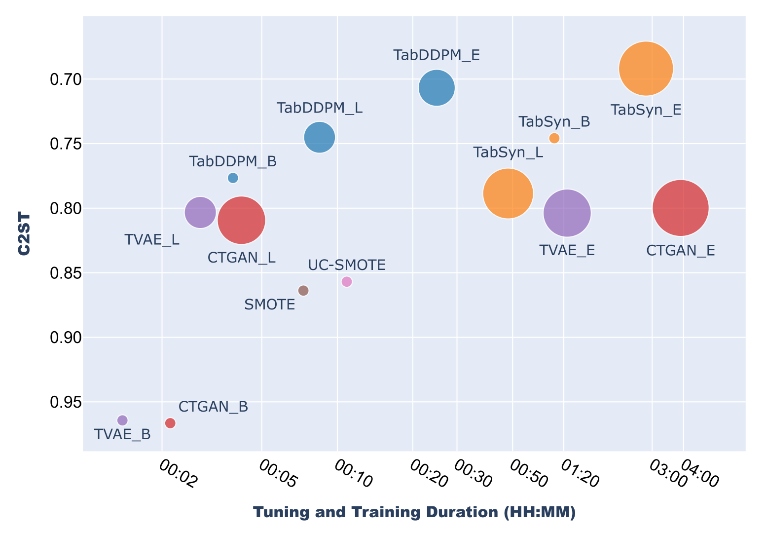
Figure 10: Average C2ST performance of the models under various setups (base models are appended with ” B”, limited-budget with ” L” and extensive with ” E”). The C2ST axis shows the best models at the top, the dot diameter indicates the complexity of the search space. The duration axis and dot diameters are logscaled for better visualization.

Finally, as shown in Figure 10, the costs induced by the heavily optimized TabSyn model are high compared to the base one. The performance gain and the gap in cost should be considered depending on the task and constraints as the base model already delivers decent performance.

It is worth noting that, due to its quick implementation, TabDDPM performed sometimes more training steps within its 20 minutes time budget on the limited-budget experiment than it did on the extensive search where the number of steps was bounded. But on the other hand, its performance was also affected by the reduced number of trials (50 instead of 300).

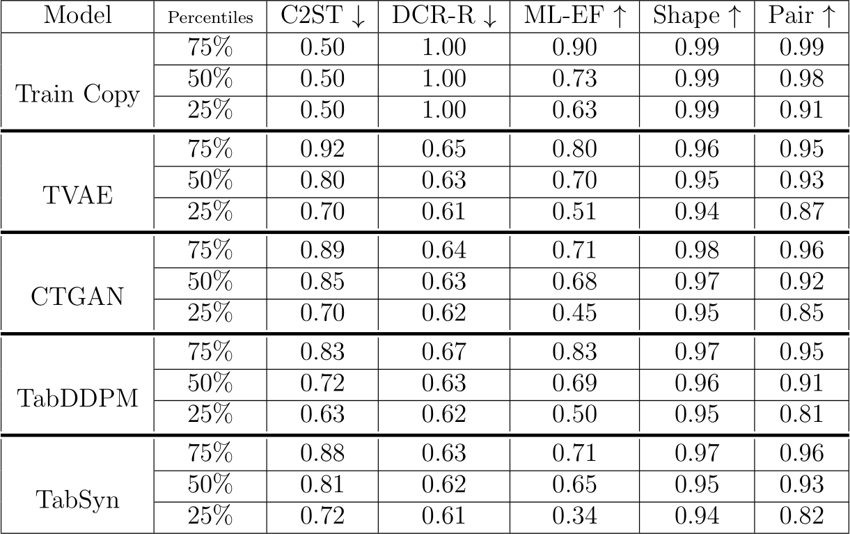
Table 5: Performance dispersion across all datasets in the limited-budget benchmark. DCR-R and ML-EF stand for DCR-Rate and ML-Efficacy respectively.

5.2.2. Multi-criteria Analysis of the Limited-Budget Tuning

In Figure 11 we summarize the model’s relative performances according to the five metrics for the limited-budget tuning experiment. To complete this point of view, Table 5 summarizes the quality metric distributions among all datasets and folds. The full results are detailed in Appendix F.

A first remark about Figure 11 is that it is more balanced than Figure 5: with a fair and limited GPU budget allocation, the models tends to perform similarly among all criteria.

There is no more clear leading model although TabDDPM obtains the best C2ST performance and TabSyn slightly dominates in terms of privacy (DCR-Rate). We however have a safe median DCR-Rate score of about 0.63 for this experiment on all neural models (against 0.62 for the extensive experiment). For ML-Efficacy, TabDDPM remains slightly the best but there is no clear leader either.

The reduced search space that we provide is hence a good starting point to perform a quick dataset-specific hyperparameters optimization that will fit on a medium-size workstation.

The relatively balanced results of this new experiment confirms that the superiority of a tabular data generator is not only due to its model but also to the whole tuning and training compute effort.

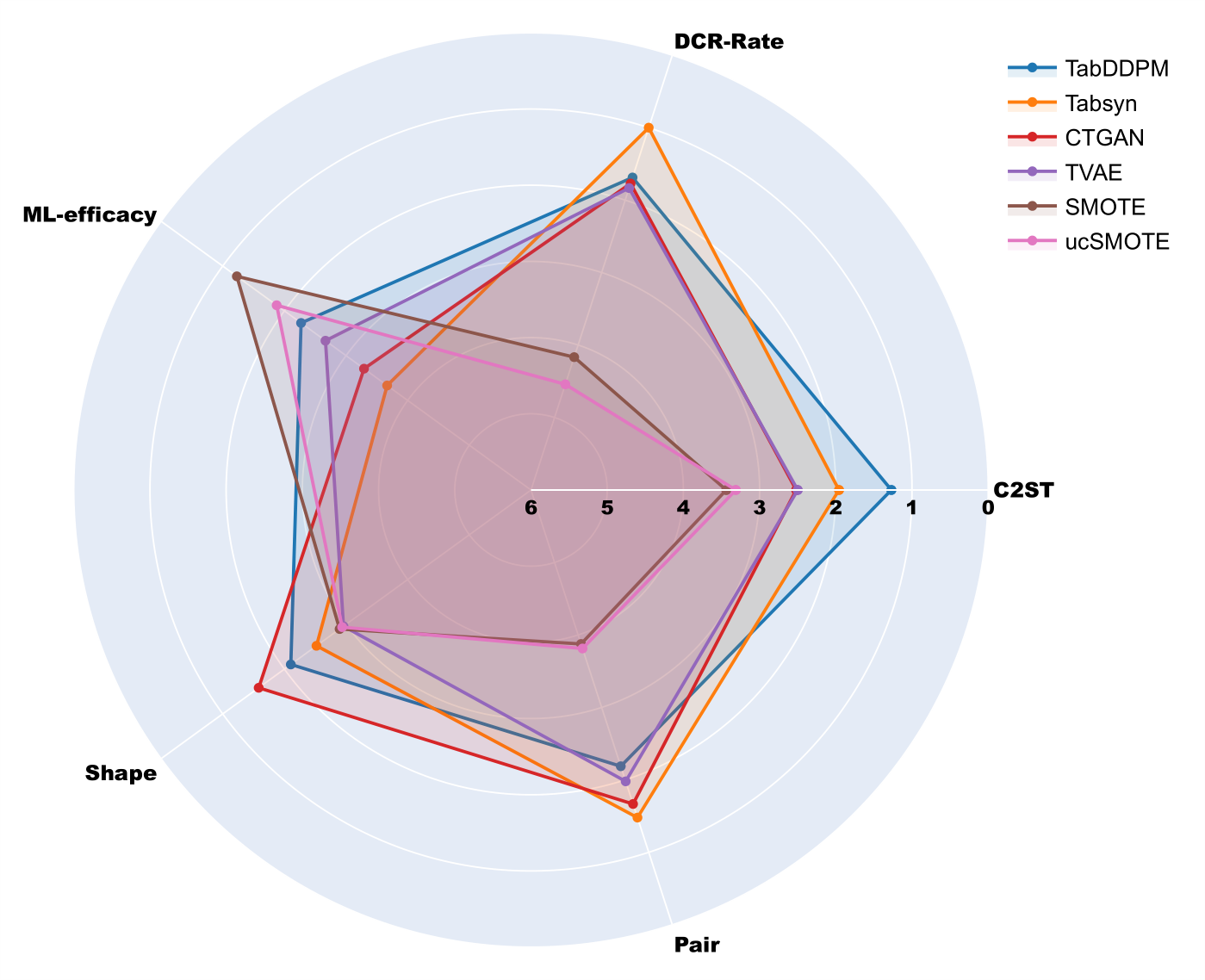
Figure 11: Radar chart of the optimized models in the limited-budget benchmark across various metrics. ”Shape” stands for column-wise similarity, and ”Pair” stands for pair-wise correlation.

Overall, TabDDPM provides a good balance between realism, privacy, utility, and cost. TVAE is a viable alternative if the utility constraint can be relaxed. It can be tuned using the limited-budget experiment search space to quickly achieve good performance. If resources are available and cost is not a priority, it is advisable to tune TabSyn, which achieves good realism results but at a higher cost. Finally, for quick results when privacy is not a concern and when the main focus is utility, SMOTE is the recommended approach.

We proposed a typology of state-of-art models for tabular data generation and we benchmarked five of them on 16 datasets with a strict 3-fold cross-validation procedure. The number of folds was limited to 3 because increasing it would have dramatically increased the costs and carbon footprint. We performed extensive large-scale tuning on a super computer from which we derived a reduced search-space. Moreover, we performed a limited-budget benchmark that fits on a medium-size workstation. Leveraging these benchmarks we were able to provide several insights on the models while answering to three technical questions: (i) is it worth optimizing the hyperparameters/preprocessing specifically for each dataset? (ii) can we propose a reduced search space that fits well for all datasets? (iii) is there a clear trade-off between training/sampling costs, and synthetic data quality?

For the two first questions, Figure 10 is certainly the best summary: most models, including TabSyn, benefit greatly from a dataset-specific tuning. However, the whole tuning process is costly in terms of time, money, energy, and COemissions, and there is clearly a ”diminishing return” effect. We conclude that, even for TabSyn, a quick dataset-specific model tuning based on the reduced search spaces we provide in Appendix A is enough to get most of the performance at the scale of a medium-size workstation. We also recommend using a subset of the dataset for hyperparameter tuning. The obtained hyperparameters can then be used to train the model at full-scale.

Regarding the trade-off question on the multiple considered criteria: realism, privacy, utility and costs, Figure 5 and Figure 11 confirm that if we do not limit the compute power, the two diffusion-based models TabDDPM and TabSyn are the most recommended solutions for tabular data generation. Nevertheless, the performance gaps between models become quite narrow with a limited compute power.

Our study focuses on models trained, tuned, and evaluated on a single table and can be extended to evaluate cross-table models that fits with multiple table structures. This is an important step towards foundation models for tabular data generation. Models such as GReaT [38] offers an interesting approach for a cross-table approach by converting the data generation process into a text generation one. However, when evaluated on a single tables, it struggle against models like CTGAN [20] for joint probability distribution [15, 11]. Working on a cross-table foundation model also introduces additional considerations towards data poisoning or adversarial attacks as foundation models are proned to being poisoned [79].

Another important research direction is the models’ interpretability. Understanding the generation procedure is also important to build user’s trust for decision making. Such interpretability study can be performed starting from a tree-based model such as Forest-Flow [63].

This work was granted access to the HPC resources of IDRIS under the allocations 2023-AD011014381, 2023-AD011011407R3, and 2023-AD011012220R2 made by GENCI.

[1] D. Libes, D. Lechevalier, S. Jain, Issues in synthetic data generation for advanced manufacturing, in: 2017 IEEE International Conference on Big Data (Big Data), IEEE, 2017, pp. 1746–1754.

[2] V. Borisov, T. Leemann, K. Seßler, J. Haug, M. Pawelczyk, G. Kasneci, Deep neural networks and tabular data: A survey, IEEE Transactions on Neural Networks and Learning Systems (2022).

[3] L. Zhang, S. Zhang, K. Balog, Table2vec: Neural word and entity embeddings for table population and retrieval, in: Proceedings of the 42nd international ACM SIGIR conference on research and development in information retrieval, 2019, pp. 1029–1032.

[4] S. Chitlangia, A. Muralidhar, R. Agarwal, Self supervised pre-training for large scale tabular data, in: NeurIPS 2022 Workshop on Table Representation Learning, 2022.

[5] T. Zhang, S. Wang, S. Yan, L. Jian, Q. Liu, Generative table pre-training empowers models for tabular prediction, in: H. Bouamor, J. Pino, K. Bali (Eds.), Proceedings of the 2023 Conference on Empirical Methods in Natural Language Processing, Association for Computational Linguistics, Singapore, 2023, pp. 14836–14854. URL: https: //aclanthology.org/2023.emnlp-main.917. doi:10.18653/v1/2023 .emnlp-main.917.

[6] L. Grinsztajn, E. Oyallon, G. Varoquaux, Why do tree-based models still outperform deep learning on typical tabular data?, in: Thirtysixth Conference on Neural Information Processing Systems Datasets and Benchmarks Track, 2022. URL: https://openreview.net/forum ?id=Fp7__phQszn.

[7] C. M. Bowen, J. Snoke, Comparative study of differentially private synthetic data algorithms from the nist pscr differential privacy synthetic data challenge, Journal of Privacy and Confidentiality 11 (2021). URL: https://journalprivacyconfidentiality.org/index.php/jpc/ar ticle/view/748. doi:10.29012/jpc.748.

[8] C. Arnold, M. Neunhoeffer, Really useful synthetic data–a framework to evaluate the quality of differentially private synthetic data, arXiv e-prints (2020) arXiv–2004.

[9] Y. Tao, R. McKenna, M. Hay, A. Machanavajjhala, G. Miklau, Bench- marking differentially private synthetic data generation algorithms (2022).

[10] Y. Hu, F. Wu, Q. Li, Y. Long, G. Garrido, C. Ge, B. Ding, D. Forsyth, B. Li, D. Song, Sok: Privacy-preserving data synthesis, in: 2024 IEEE Symposium on Security and Privacy (SP), IEEE Computer Society, 2023, pp. 2–2.

[11] Y. Du, N. Li, Towards principled assessment of tabular data synthesis algorithms, arXiv preprint arXiv:2402.06806 (2024).

[12] G. Zab¨ergja, A. Kadra, J. Grabocka, Tabular data: Is attention all you need?, 2024. arXiv:2402.03970.

[13] J. Fonseca, F. Bacao, Tabular and latent space synthetic data genera- tion: a literature review, Journal of Big Data 10 (2023) 115.

[14] A. Kotelnikov, D. Baranchuk, I. Rubachev, A. Babenko, Tabddpm: Modelling tabular data with diffusion models, in: International Conference on Machine Learning, PMLR, 2023, pp. 17564–17579.

[15] H. Zhang, J. Zhang, Z. Shen, B. Srinivasan, X. Qin, C. Faloutsos, H. Rangwala, G. Karypis, Mixed-type tabular data synthesis with score-based diffusion in latent space, in: The Twelfth International Conference on Learning Representations, 2024.

[16] X. Fang, W. Xu, F. A. Tan, J. Zhang, Z. Hu, Y. Qi, S. Nickleach, D. Socolinsky, S. Sengamedu, C. Faloutsos, Large language models on tabular data–a survey, arXiv preprint arXiv:2402.17944 (2024).

[17] D. P. Kingma, M. Welling, Auto-encoding variational bayes, stat 1050 (2014) 1.

[18] I. Goodfellow, J. Pouget-Abadie, M. Mirza, B. Xu, D. Warde-Farley, S. Ozair, A. Courville, Y. Bengio, Generative adversarial networks, Communications of the ACM 63 (2020) 139–144.

[19] E. G. Tabak, C. V. Turner, A family of nonparametric density estima- tion algorithms, Communications on Pure and Applied Mathematics 66 (2013) 145–164.

[20] L. Xu, M. Skoularidou, A. Cuesta-Infante, K. Veeramachaneni, Model- ing tabular data using conditional gan, in: H. Wallach, H. Larochelle, A. Beygelzimer, F. d'Alch´e-Buc, E. Fox, R. Garnett (Eds.), Advances in Neural Information Processing Systems (NeurIPS), volume 32, Curran Associates, Inc., 2019.

[21] N. Patki, R. Wedge, K. Veeramachaneni, The synthetic data vault, in: IEEE International Conference on Data Science and Advanced Analytics (DSAA), 2016, pp. 399–410. doi:10.1109/DSAA.2016.49.

[22] C. Ma, S. Tschiatschek, R. Turner, J. M. Hern´andez-Lobato, C. Zhang, Vaem: a deep generative model for heterogeneous mixed type data, Advances in Neural Information Processing Systems 33 (2020) 11237– 11247.

[23] Z. Zhao, A. Kunar, R. Birke, L. Y. Chen, Ctab-gan: Effective table data synthesizing, in: Asian Conference on Machine Learning, PMLR, 2021, pp. 97–112.

[24] E. H. Zein, T. Urvoy, Tabular data generation: Can we fool XGBoost ?, in: NeurIPS 2022 First Table Representation Workshop, 2022.

[25] L. V. H. Vardhan, S. Kok, Generating privacy-preserving synthetic tabular data using oblivious variational autoencoders, in: Proceedings of the Workshop on Economics of Privacy and Data Labor at the 37 th International Conference on Machine Learning, 2020.

[26] T. Liu, Z. Qian, J. Berrevoets, M. van der Schaar, GOGGLE: Generative modelling for tabular data by learning relational structure, in: The Eleventh International Conference on Learning Representations, 2023. URL: https://openreview.net/forum?id=fPVRcJqspu.

[27] J. Jordon, J. Yoon, M. van der Schaar, Pate-gan: Generating synthetic data with differential privacy guarantees, in: International Conference on Learning Representations, 2018. URL: https://api.semanticscho lar.org/CorpusID:53342261.

[28] N. Park, M. Mohammadi, K. Gorde, S. Jajodia, H. Park, Y. Kim, Data synthesis based on generative adversarial networks, Proceedings of the VLDB Endowment 11 (2018).

[29] R. D. Camino, C. Hammerschmidt, et al., Generating multi-categorical samples with generative adversarial networks, in: ICML 2018 workshop on Theoretical Foundations and Applications of Deep Generative Models, 2018.

[30] M. K. Baowaly, C.-C. Lin, C.-L. Liu, K.-T. Chen, Synthesizing electronic health records using improved generative adversarial networks, Journal of the American Medical Informatics Association: JAMIA 26 (2019) 228–241.

[31] H. Chen, S. Jajodia, J. Liu, N. Park, V. Sokolov, V. Subrahmanian, Faketables: Using gans to generate functional dependency preserving tables with bounded real data, in: 28th International Joint Conference on Artificial Intelligence, IJCAI 2019, International Joint Conferences on Artificial Intelligence, 2019, pp. 2074–2080.

[32] A. Koivu, M. Sairanen, A. Airola, T. Pahikkala, Synthetic minority oversampling of vital statistics data with generative adversarial networks, Journal of the American Medical Informatics Association 27 (2020) 1667–1674.

[33] R. Sauber-Cole, T. M. Khoshgoftaar, The use of generative adversarial networks to alleviate class imbalance in tabular data: a survey, Journal of Big Data 9 (2022) 98.

[34] D. S. Watson, K. Blesch, J. Kapar, M. N. Wright, Adversarial random forests for density estimation and generative modeling, in: International

Conference on Artificial Intelligence and Statistics, PMLR, 2023, pp. 5357–5375.

[35] M. Arjovsky, S. Chintala, L. Bottou, Wasserstein generative adversarial networks, in: International conference on machine learning, PMLR, 2017, pp. 214–223.

[36] S. Bond-Taylor, A. Leach, Y. Long, C. G. Willcocks, Deep generative modelling: A comparative review of vaes, gans, normalizing flows, energy-based and autoregressive models, IEEE Transactions on Pattern Analysis and Machine Intelligence 44 (2022) 7327–7347. doi:10.1109/TPAMI.2021.3116668.

[37] L. Ouyang, J. Wu, X. Jiang, D. Almeida, C. Wainwright, P. Mishkin, C. Zhang, S. Agarwal, K. Slama, A. Gray, J. Schulman, J. Hilton, F. Kelton, L. Miller, M. Simens, A. Askell, P. Welinder, P. Christiano, J. Leike, R. Lowe, Training language models to follow instructions with human feedback, in: A. H. Oh, A. Agarwal, D. Belgrave, K. Cho (Eds.), Advances in Neural Information Processing Systems, 2022. URL: https://openreview.net/forum?id=TG8KACxEON.

[38] V. Borisov, K. Sessler, T. Leemann, M. Pawelczyk, G. Kasneci, Lan- guage models are realistic tabular data generators, in: The Eleventh International Conference on Learning Representations (ICLR), 2023.

[39] A. Radford, J. Wu, R. Child, D. Luan, D. Amodei, I. Sutskever, Lan- guage models are unsupervised multitask learners, OpenAI (2019). URL: https://cdn.openai.com/better-language-models/language_mod els_are_unsupervised_multitask_learners.pdf, accessed: 2024-11-15.

[40] A. V. Solatorio, O. Dupriez, Realtabformer: Generating realistic relational and tabular data using transformers, arXiv preprint arXiv:2302.02041 (2023).

[41] J. Sohl-Dickstein, E. Weiss, N. Maheswaranathan, S. Ganguli, Deep unsupervised learning using nonequilibrium thermodynamics, in: International Conference on Machine Learning, PMLR, 2015, pp. 2256–2265.

[42] J. Ho, A. Jain, P. Abbeel, Denoising diffusion probabilistic models, Advances in neural information processing systems 33 (2020) 6840–6851.

[43] Y. Song, J. Sohl-Dickstein, D. P. Kingma, A. Kumar, S. Ermon, B. Poole, Score-based generative modeling through stochastic differential equations, in: International Conference on Learning Representations, 2021. URL: https://openreview.net/forum?id=PxTIG12RRHS.

[44] P. Dhariwal, A. Nichol, Diffusion models beat gans on image synthesis, Advances in neural information processing systems 34 (2021) 8780–8794.

[45] T. Karras, M. Aittala, T. Aila, S. Laine, Elucidating the design space of diffusion-based generative models, Advances in Neural Information Processing Systems 35 (2022) 26565–26577.

[46] G. Truda, Generating tabular datasets under differential privacy, arXiv preprint arXiv:2308.14784 (2023). TableDiffusion.

[47] J. Kim, C. Lee, N. Park, STaSy: Score-based tabular data synthesis (2022).

[48] C. Lee, J. Kim, N. Park, Codi: Co-evolving contrastive diffusion models for mixed-type tabular synthesis, in: Proceedings of the 40th International Conference on Machine Learning, ICML’23, JMLR.org, 2023.

[49] A. Vahdat, K. Kreis, J. Kautz, Score-based generative modeling in latent space, Advances in neural information processing systems 34 (2021) 11287–11302.

[50] R. Rombach, A. Blattmann, D. Lorenz, P. Esser, B. Ommer, Highresolution image synthesis with latent diffusion models, in: Proceedings of the IEEE/CVF conference on computer vision and pattern recognition, 2022, pp. 10684–10695.

[51] R. B. Nelsen, An Introduction to Copulas, second ed., Springer, New York, NY, USA, 2006.

[52] Z. Li, Y. Zhao, J. Fu, Sync: A copula based framework for generating synthetic data from aggregated sources, in: 2020 International Conference on Data Mining Workshops (ICDMW), IEEE, 2020, pp. 571–578.

[53] S. Kamthe, S. Assefa, M. Deisenroth, Copula flows for synthetic data generation, arXiv preprint arXiv:2101.00598 (2021).

[54] D. Meyer, T. Nagler, Synthia: multidimensional synthetic data genera- tion in python, Journal of Open Source Software 6 (2021) 2863. URL: https://doi.org/10.21105/joss.02863. doi:10.21105/joss.02863.

[55] D. Meyer, T. Nagler, R. J. Hogan, Copula-based synthetic data augmen- tation for machine-learning emulators, Geoscientific Model Development 14 (2021) 5205–5215. URL: https://doi.org/10.5194/gmd-14-520 5-2021. doi:10.5194/gmd-14-5205-2021.

[56] R. Mckenna, D. Sheldon, G. Miklau, Graphical-model based estimation and inference for differential privacy, in: K. Chaudhuri, R. Salakhutdinov (Eds.), Proceedings of the 36th International Conference on Machine Learning, volume 97 of Proceedings of Machine Learning Research, PMLR, 2019, pp. 4435–4444. URL: https://proceedings.mlr.pres s/v97/mckenna19a.html.

[57] Z. Zhang, T. Wang, N. Li, J. Honorio, M. Backes, S. He, J. Chen, Y. Zhang, {PrivSyn}: Differentially private data synthesis, in: 30th USENIX Security Symposium (USENIX Security 21), 2021, pp. 929– 946.

[58] J. Dahmen, D. J. Cook, Synsys: A synthetic data generation system for healthcare applications, Sensors (Basel, Switzerland) 19 (2019). URL: https://api.semanticscholar.org/CorpusID:75136844.

[59] B. Tang, H. He, Kerneladasyn: Kernel based adaptive synthetic data generation for imbalanced learning, in: 2015 IEEE Congress on Evolutionary Computation (CEC), 2015, pp. 664–671. doi:10.1109/CEC.20 15.7256954.

[60] M. Baak, S. Brugman, I. Fridman Rojas, L. Dalmeida, R. E.Q. Urlus, J.-B. Oger, Synthsonic: Fast, probabilistic modeling and synthesis of tabular data, in: G. Camps-Valls, F. J. R. Ruiz, I. Valera (Eds.), Proceedings of The 25th International Conference on Artificial Intelligence and Statistics, volume 151 of Proceedings of Machine Learning Research, PMLR, 2022, pp. 4747–4763. URL: https://proceedings.mlr.pres s/v151/baak22a.html.

[61] R. McKenna, G. Miklau, D. Sheldon, Winning the nist contest: A scalable and general approach to differentially private synthetic data,

Journal of Privacy and Confidentiality 11 (2021). URL: https://journa lprivacyconfidentiality.org/index.php/jpc/article/view/778. doi:10.29012/jpc.778.

[62] J. Jewson, L. Li, L. Battaglia, S. Hansen, D. Rossell, P. Zwiernik, Graph- ical model inference with external network data, cemmap working paper CWP20/22, London, 2022. URL: https://hdl.handle.net/10419/2 72832. doi:10.47004/wp.cem.2022.2022.

[63] A. Jolicoeur-Martineau, K. Fatras, T. Kachman, Generating and im- puting tabular data via diffusion and flow-based gradient-boosted trees, in: S. Dasgupta, S. Mandt, Y. Li (Eds.), Proceedings of The 27th International Conference on Artificial Intelligence and Statistics, volume 238 of Proceedings of Machine Learning Research, PMLR, 2024, pp. 1288– 1296. URL: https://proceedings.mlr.press/v238/jolicoeur-mar tineau24a.html.

[64] N. V. Chawla, K. W. Bowyer, L. O. Hall, W. P. Kegelmeyer, Smote: synthetic minority over-sampling technique, Journal of artificial intelligence research 16 (2002) 321–357.

[65] L. Torgo, R. Ribeiro, B. Pfahringer, P. Branco, Smote for regression, volume 8154, 2013, pp. 378–389. doi:10.1007/978-3-642-40669-0_33.

[66] L. Camacho, G. Douzas, F. Bacao, Geometric smote for regression, Expert Systems with Applications 193 (2022) 1–8. doi:10.1016/j.eswa .2021.116387, camacho, L., Douzas, G., & Bacao, F. (2022). Geometric SMOTE for regression. Expert Systems with Applications, 193(May), 1-8. [116387]. https://doi.org/10.1016/j.eswa.2021.116387.

[67] D. Lopez-Paz, M. Oquab, Revisiting classifier two-sample tests, in: International Conference on Learning Representations, 2016.

[68] T. Chen, C. Guestrin, Xgboost: A scalable tree boosting system, in: Proceedings of the 22nd acm sigkdd international conference on knowledge discovery and data mining, 2016, pp. 785–794.

[69] L. Prokhorenkova, G. Gusev, A. Vorobev, A. V. Dorogush, A. Gulin, Catboost: unbiased boosting with categorical features, Advances in neural information processing systems 31 (2018).

[70] M. Platzer, T. Reutterer, Holdout-based empirical assessment of mixed- type synthetic data, Frontiers in big Data 4 (2021) 679939.

[71] R. Liaw, E. Liang, R. Nishihara, P. Moritz, J. E. Gonzalez, I. Stoica, Tune: A research platform for distributed model selection and training, arXiv preprint arXiv:1807.05118 (2018).

[72] J. Bergstra, D. Yamins, D. Cox, Making a science of model search: Hyperparameter optimization in hundreds of dimensions for vision architectures, in: International conference on machine learning, PMLR, 2013, pp. 115–123.

[73] J. Bergstra, R. Bardenet, Y. Bengio, B. K´egl, Algorithms for hyper- parameter optimization, in: J. Shawe-Taylor, R. Zemel, P. Bartlett, F. Pereira, K. Weinberger (Eds.), Advances in Neural Information Processing Systems, volume 24, Curran Associates, Inc., 2011. URL: https://proceedings.neurips.cc/paper_files/paper/2011/file /86e8f7ab32cfd12577bc2619bc635690-Paper.pdf.

[74] L. Li, K. Jamieson, A. Rostamizadeh, E. Gonina, J. Ben-tzur, M. Hardt, B. Recht, A. Talwalkar, A system for massively parallel hyperparameter tuning, in: I. Dhillon, D. Papailiopoulos, V. Sze (Eds.), Proceedings of Machine Learning and Systems, volume 2, 2020, pp. 230–246. URL: https://proceedings.mlsys.org/paper_files/paper/2020/file/ a06f20b349c6cf09a6b171c71b88bbfc-Paper.pdf.

[75] Y. Gorishniy, I. Rubachev, A. Babenko, On embeddings for numeri- cal features in tabular deep learning, Advances in Neural Information Processing Systems 35 (2022) 24991–25004.

[76] P. K. Dunn, G. K. Smyth, Randomized quantile residuals, Journal of Computational and graphical statistics 5 (1996) 236–244.

[77] P. Mettes, E. van der Pol, C. G. M. Snoek, Hyperspherical Prototype Networks, Curran Associates Inc., Red Hook, NY, USA, 2019.

[78] J. Demˇsar, Statistical comparisons of classifiers over multiple data sets, The Journal of Machine learning research 7 (2006) 1–30.

[79] A. Wan, E. Wallace, S. Shen, D. Klein, Poisoning language models during instruction tuning, in: Proceedings of the 40th International Conference on Machine Learning, ICML’23, JMLR.org, 2023.

Hyperparameters search space of TVAE is in Table A.6, for CTGAN in A.7, for TabSyn’s VAE and MLP in A.8, for TabDDPM in A.9, for smote and ucsmote in A.10. These tables also present the reduced search spaces suggested and applied for the experiment of Section 5.

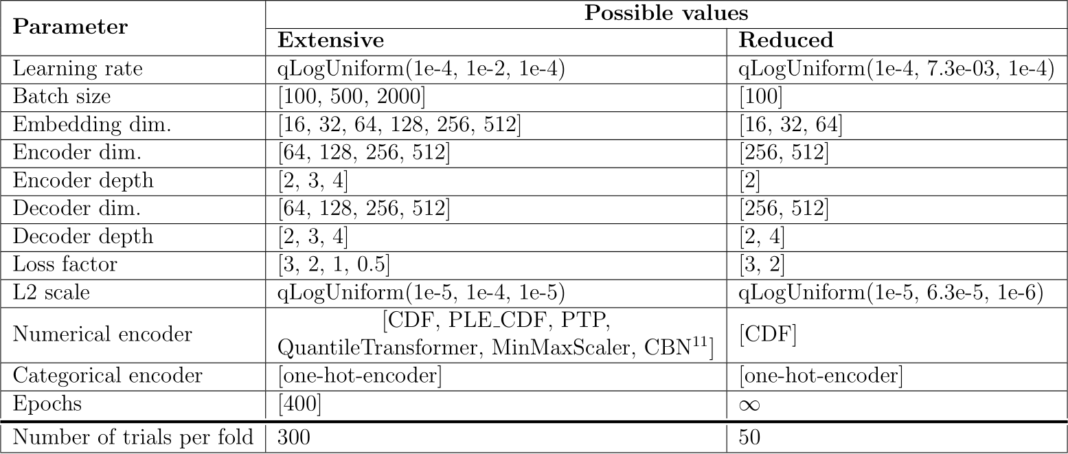
Table A.6: Hyperparameter search spaces of TVAE: extensive and limited-budget benchmarks.

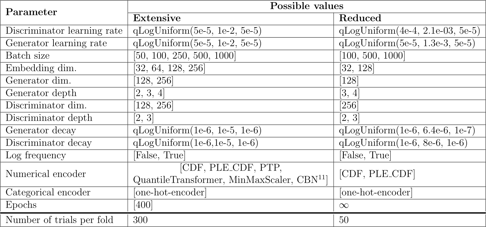
Table A.7: Hyperparameter search spaces of CTGAN for the extensive and limited-budget benchmarks.

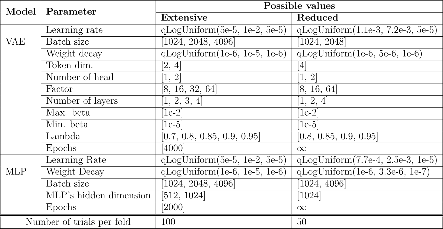
Table A.8: Hyperparameter search spaces of TabSyn’s VAE and MLP for the extensive and limited-budget benchmarks. In the second benchmark, the number of epochs was bounded by a time budget (10 minutes for the VAE, 10 minutes for the denoiser).

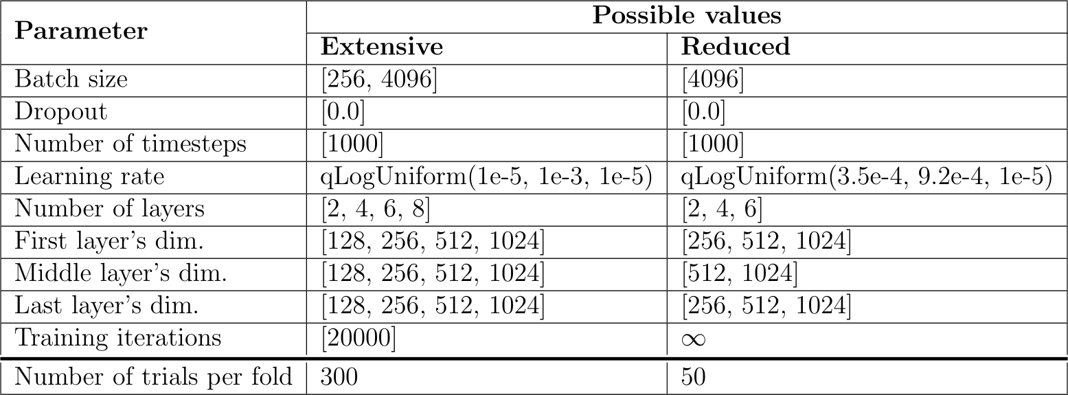
Table A.9: Hyperparameter search spaces of TabDDPM for the extensive and limited-budget benchmarks.

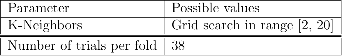
Table A.10: Hyperparameter search space of SMOTE and ucSMOTE.

We provide the list of links toward the datasets that were used in this paper in Table B.11 below.

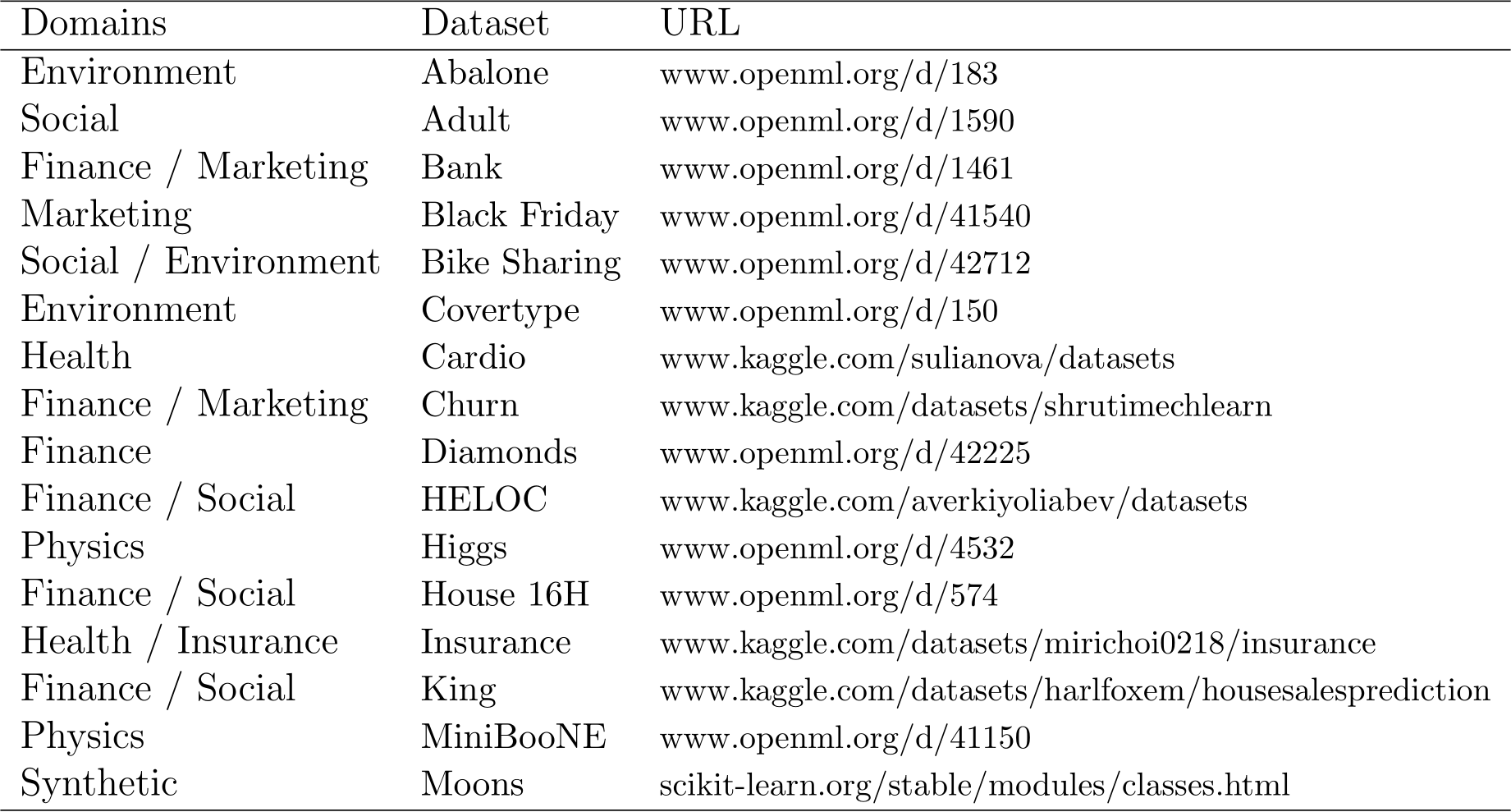
Table B.11: Domains and links to the datasets

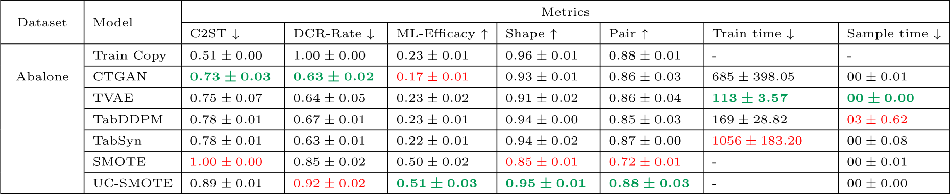
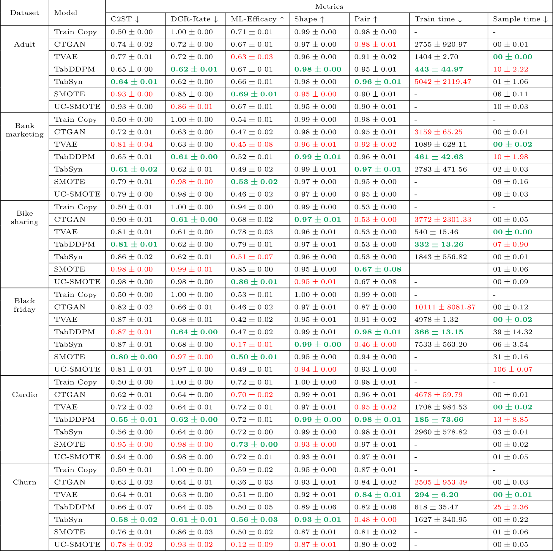
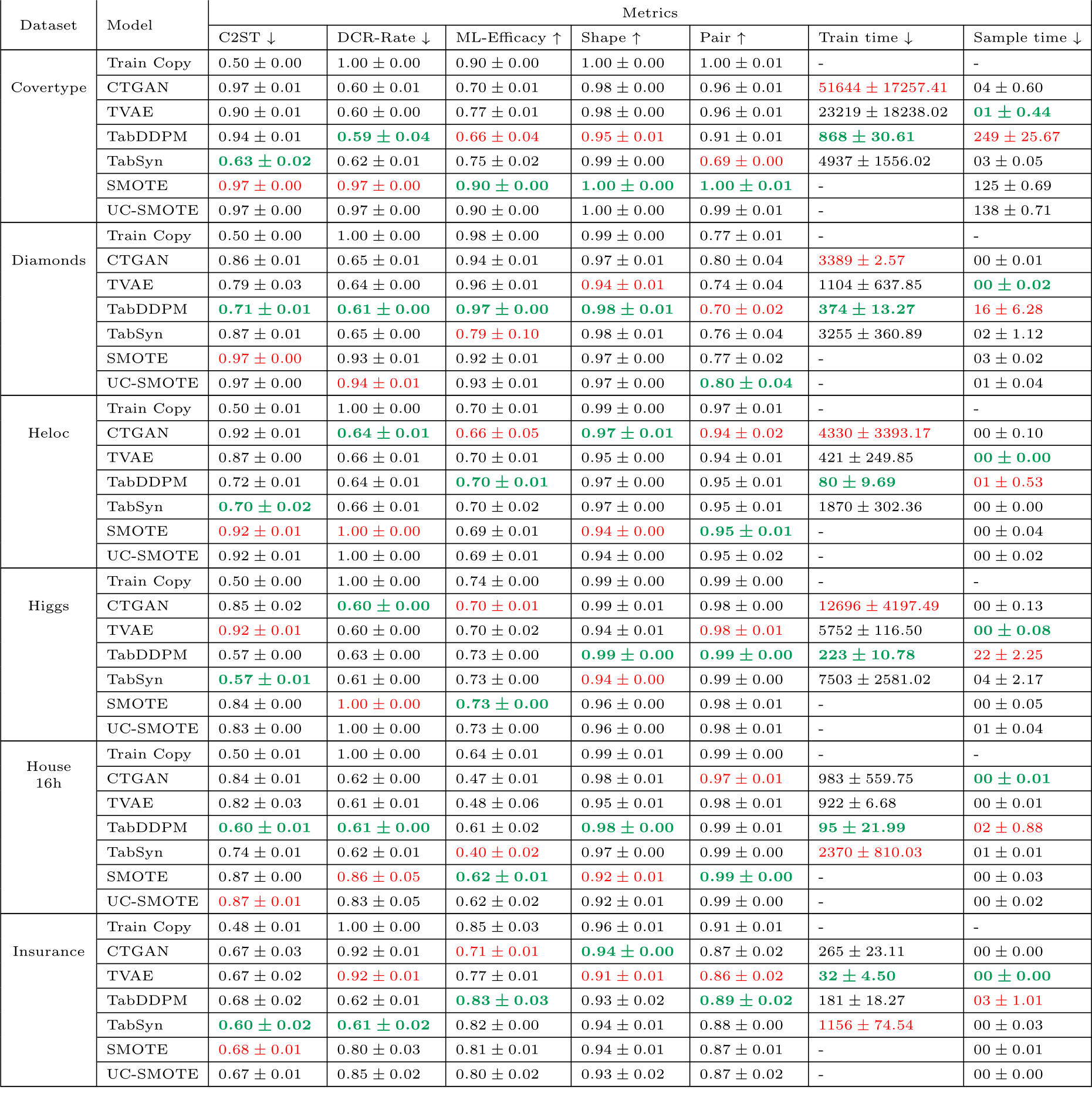
Table C.12 present the per-dataset performance according to the metrics described in Section 3.2 averaged on 3-folds with 5 samples per-fold.

Results per datasets and models under diverse metrics for the extensive search (continued).

Results per datasets and models under diverse metrics for the extensive search (continued).

Results per datasets and models under diverse metrics for the extensive search (continued).

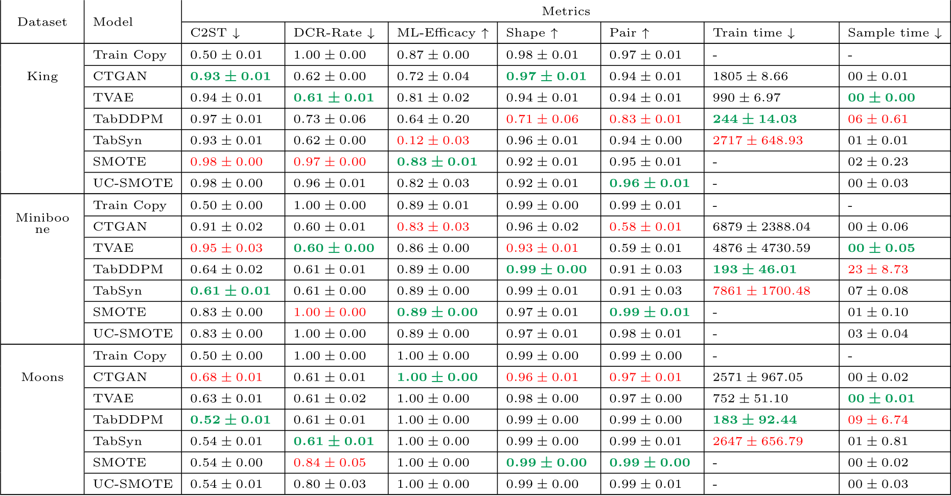
Table C.12: Results per dataset and model under diverse metrics. The training times (gradient descent) and sampling times are given in seconds. The sampling times are given for 5 samples. The best values per metric are formatted in bold green and the worse values are in red.

We performed large-scale experiments including a quite costly hyperparameter tuning step. Note that the term ”costs” in this section refers to the duration, energy consumption, and COemissions. We evaluate the training and sampling costs of the models with their optimized hyperparameters, as well as the full hyperparameter tuning costs.

Appendix D.1. Training and Sampling Costs

Due to the massive nature of the experiments, the hyperparameter search could not all be run on the same hardware. We hence estimated the training (gradient descent) cost by running all models on a single Tesla V100-SXM2 32 GB. Table D.13 provides the raw training and sampling energy consumption and emissions for reference. All of the TabSyn costs shown are a combination of the VAE cost and the denoiser cost, which are estimated separately and then added together. Also, all TabSyn costs on the Covertype dataset are estimated considering the complete dataset size.

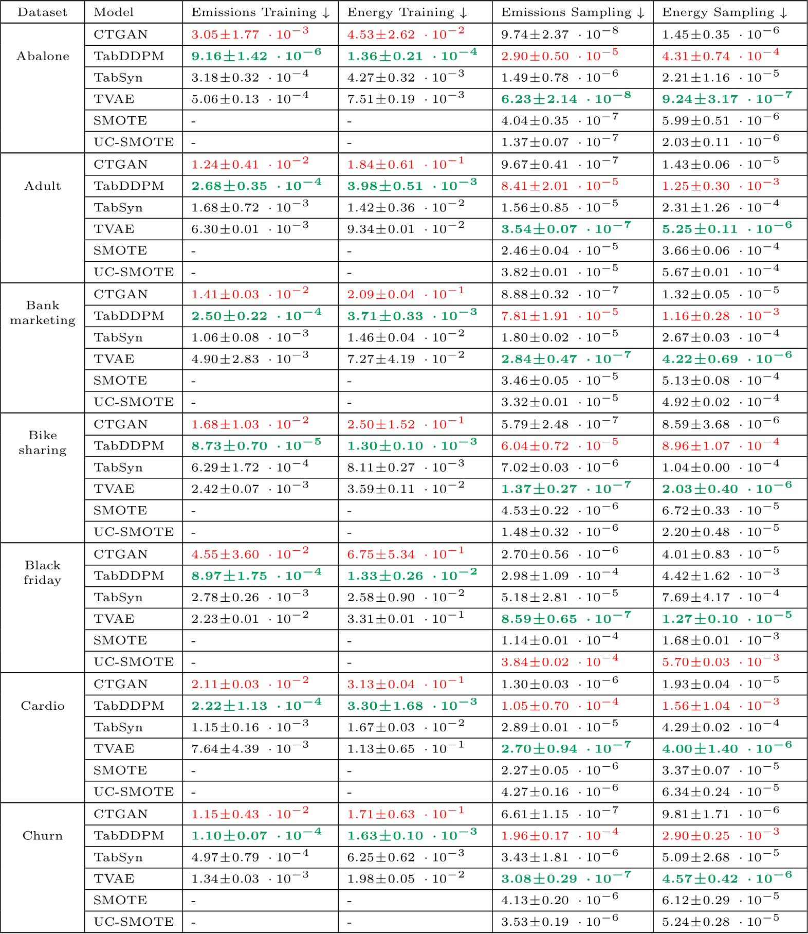
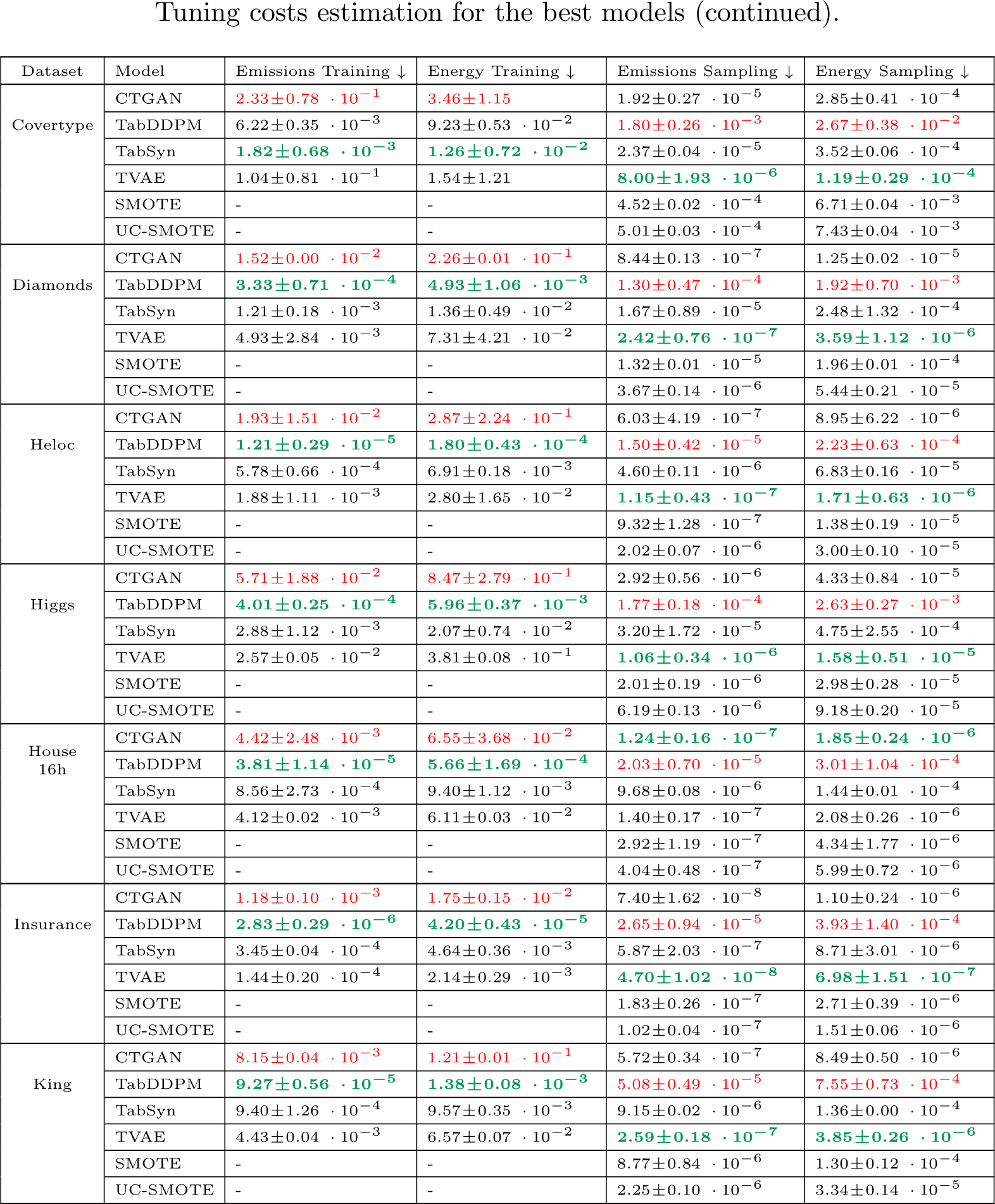
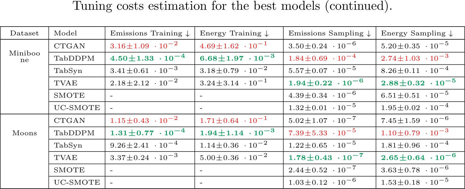
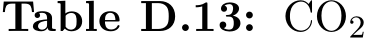emissions (in Kg) and Energy Consumption (in kWh) of the benchmark challengers. The energy consumption is obtained by summing the CPU, GPU and RAM energy. Training costs are given for all models on the same basis of 400 epochs. Sampling costs are given for 5 samples. The best values are formatted in bold green and the worse are in red.

Appendix D.2. Whole Tuning Cost Estimation

As mentioned in Section 3.2 we could not perform the hyperparameter search and training phases on a uniform hardware and software architecture and we estimated the tuning cost with Equation (1).

Each trial can be stopped based on three conditions: an early stopping decided by the model, a poor C2ST performance or a time limit. Therefore, to get an accurate estimate of the init-cost and the cost-per-step from the single-GPU mentioned in Appendix D.1, we needed to extract from our logs the effective number of training steps performed per trial.

In addition, we also considered the parallelization scheme applied during the tuning procedure. One issue with TabSyn was that we observed a general slowdown when the model was parallelized too heavily. This issue was even more marked on datasets with a large number of columns. We hence reduced the number trials per GPU and the global number of trials to 100 to fall back to a reasonable time for this model.

Finally, we measured cost on a typical configuration used during our tuning experiment: 8 Tesla V100-SXM2 32 GB. Considering those 8 GPUs, we used the following parallel allocation of trials: 64 for TVAE and CTGAN, 40 for TabDDPM, and 16 for TabSyn. A model that can be easily parallelized during the hyperparameter tuning phase offers a cost advantage. It is hence important to consider this aspect during the evaluation process. The results are presented in Table D.14.

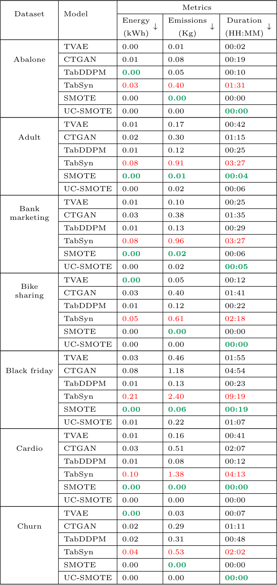
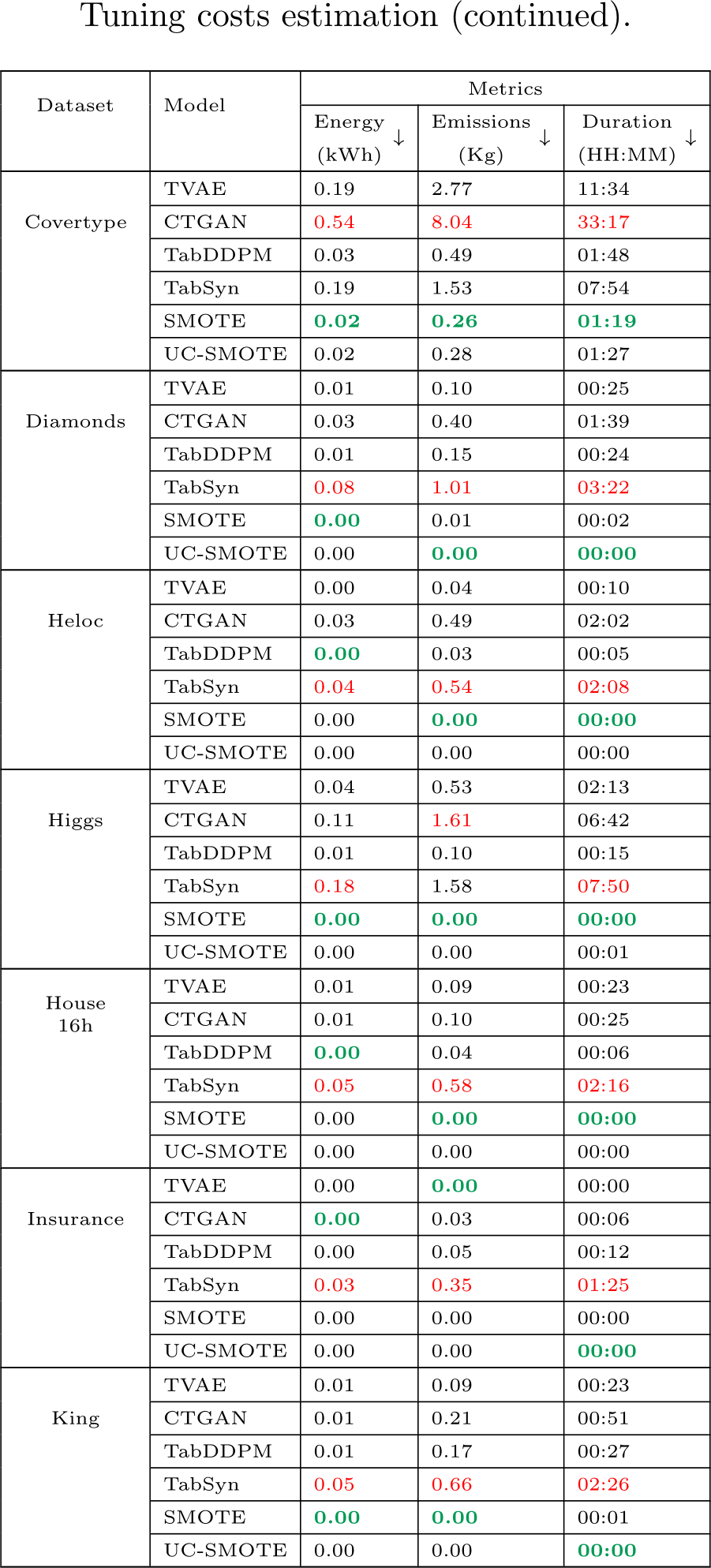
Table D.14: Estimated hyperparameter search cost based on the estimated training cost of the best models presented in Table D.13. All costs associated with TabSyn include those incurred by the VAE and the denoiser. The energy and emissions values are rounded to two decimals and take into account the number of trials we could run in parallel per model. The best values per metric are formatted in bold green and the worse are in red.

We also trained the models using their native codes and hyperparameters to provide an additional reference for comparison with their tuned versions. Table E.15 presents the results as evaluated under the same procedure as the tuned models for C2ST, DCR-Rate, ML-Efficacy, column-wise similarity (named ”Shape”), and pair-wise correlation (named ”Pair”). For TabDDPM, since there is no default hyperparameters provided [14], we fixed one based on the base configuration provided in the authors’ GitHub repository.

Results per datasets and models under diverse metrics for the base models (continued).

Results per datasets and models under diverse metrics for the base models (continued).

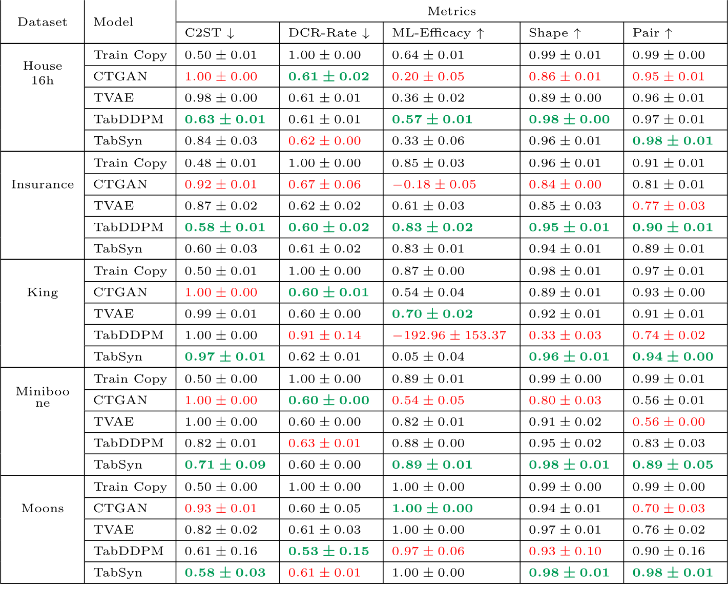
Table E.15: Results for base models. Models are trained using their default hyperparameters as provided by the authors in their papers. The best values per metric are formatted in bold green and the worse values are in red.

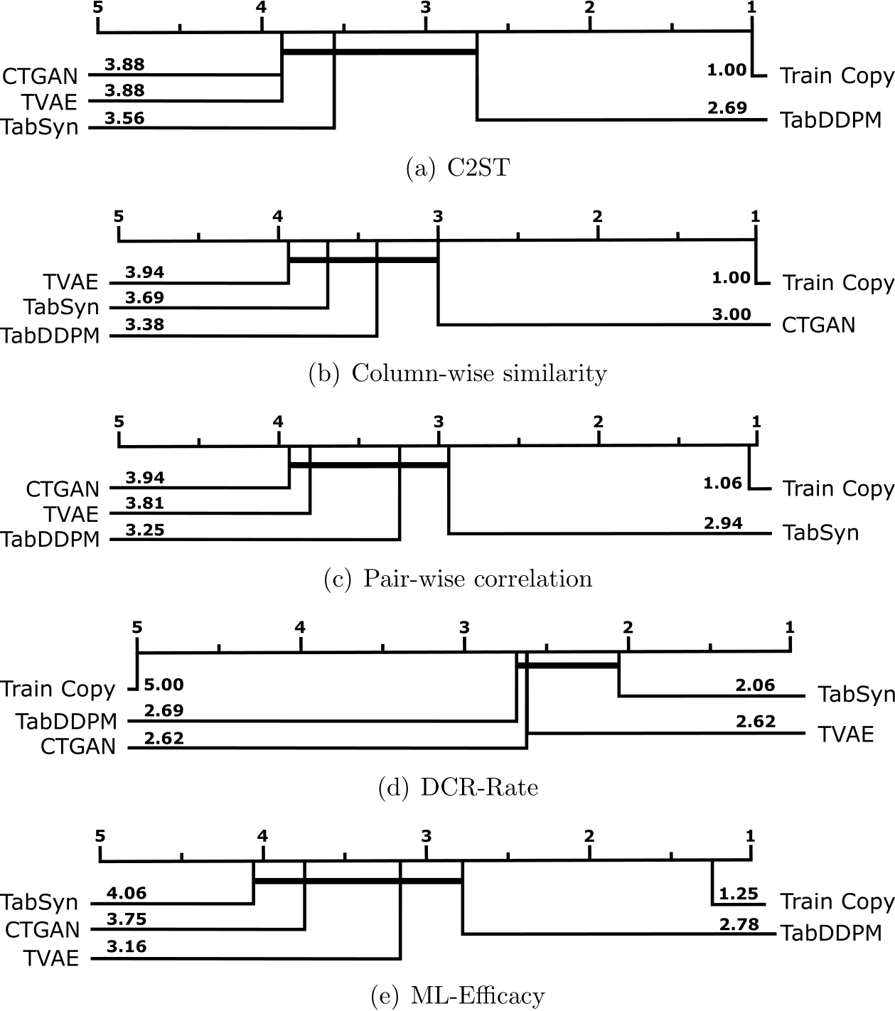
Figure F.12: Models’ ranking under the light (limited-budget) experiment setup with critical difference diagrams on C2ST, column-wise similarity, pair-wise correlation, DCR-Rate, and ML-Efficacy metrics over all datasets.

With the reduced hyperparameters search spaces presented in Appendix A, we ran a limited-budget hyperparameter tuning described in Section 5. The experiment was done on all dataset (Table 2). We performed 50 trials per fold with 3 folds, meaning we ran a total of 150 trials for this limited-budget experiment. The results par datasets are shown in Table F.16.

Results per datasets and models under diverse metrics for the limited-budget search (continued).

Results per datasets and models under diverse metrics for the limited-budget search (continued).

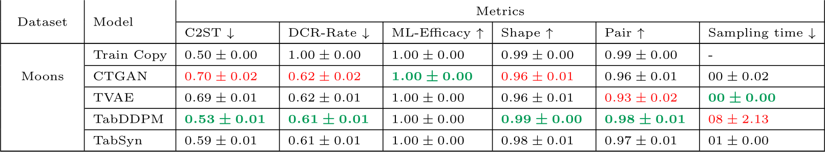
Table F.16: Limited-budget experiment results under various metrics. Results are averaged over 3 folds with 5 synthetic samples per fold as done in the extensive hyperparameter tuning. The best values per metric are formatted in bold green and the worse values are in red.